-
1. Elements
- 1.1. Element Input Format
- 1.2. Common Attributes for all Elements
- 1.3. Drift Spaces
- 1.4. Bending Magnets
- 1.5. Quadrupole
- 1.6. Sextupole
- 1.7. Octupole
- 1.8. General Multipole
- 1.9. General Multipole (will replace Section [multipole] when implemented)
- 1.10. Solenoid
- 1.11. Cyclotron
- 1.12. Ring Definition
- 1.13. Source
- 1.14. RF Cavities (OPAL-t and OPAL-cycl)
- 1.15. RF Cavities with Time Dependent Parameters
- 1.16. Traveling Wave Structure
- 1.17. Monitor
- 1.18. Collimators
- 1.19. Septum (OPAL-cycl)
- 1.20. Probe (OPAL-cycl)
- 1.21. Stripper (OPAL-cycl)
- 1.22. Degrader (OPAL-t)
- 1.23. Correctors (OPAL-t)
1. Elements
1.1. Element Input Format
All physical elements are defined by statements of the form
label:keyword, attribute,..., attribute
where
- label
-
Is the name to be given to the element (in the example QF), it is an identifier see Section [label].
- keyword
-
Is a keyword see Section [label], it is an element type keyword (in the example
QUADRUPOLE), - attribute
-
normally has the form
attribute-name=attribute-value
- attribute-name
-
selects the attribute from the list defined for the element type
keyword(in the exampleLandK1). It must be an identifier see Section [label] - attribute-value
-
gives it a value see Section [attribute] (in the example
1.8and0.015832).
Omitted attributes are assigned a default value, normally zero.
Example:
QF: QUADRUPOLE, L=1.8, K1=0.015832;
1.2. Common Attributes for all Elements
The following attributes are allowed on all elements:
- TYPE
-
A string value see Section [astring]. It specifies an "engineering type" and can be used for element selection.
- APERTURE
-
A string value see Section [astring] which describes the element aperture. All but the last attribute of the aperture have units of meter, the last one is optional and is a positive real number. Possible choices are
-
APERTURE="SQUARE(a,f)" has a square shape of width and heighta, -
APERTURE="RECTANGLE(a,b,f)" has a rectangular shape of widthaand heightb, -
APERTURE="CIRCLE(d,f)" has a circular shape of diameterd, -
APERTURE="ELLIPSE(a,b,f)" has an elliptical shape of majoraand minorb.The option
SQUARE(a,f) is equivalent toRECTANGLE(a,a,f) andCIRCLE(d,f) is equivalent toELLIPSE(d,d,f). The size of the exit aperture is scaled by a factorf. Forf < 1the exit aperture is smaller than the entrance aperture, forf = 1they are the same and forf > 1the exit aperture is bigger.Dipoles have
GAPandHGAPwhich define an aperture and hence do not recogniseAPERTURE. The aperture of the dipoles has rectangular shape of heightGAPand widthHGAP. In longitudinal direction it is bent such that its center coincides with the circular segment of the reference particle when ignoring fringe fields. Between the beginning of the fringe field and the entrance face and between the exit face and the end of the exit fringe field the rectangular shape has width and height that are twice of what they are inside the dipole.Default aperture for all other elements is a circle of 1.0m.
-
- L
-
The length of the element (default: 0m).
- WAKEF
-
Attach wakefield that was defined using the
WAKEcommand. - ELEMEDGE
-
The edge of an element is specified in s coordinates in meters. This edge corresponds to the origin of the local coordinate system and is the physical start of the element. (Note that in general the fields will extend in front of this position.) The physical end of the element is determined by
ELEMEDGEand its physical length. (Note again that in general the fields will extend past the physical end of the element.) - PARTICLEMATTERINTERACTION
-
Attach a handler for particle matter interaction, see [chp:partmatt].
- X
-
X-component of the position of the element in the laboratory coordinate system.
- Y
-
Y-component of the position of the element in the laboratory coordinate system.
- Z
-
Z-component of the position of the element in the laboratory coordinate system.
- THETA
-
Angle of rotation of the element about the y-axis relative to the default orientation,
\mathbf{n} = \left(0, 0, 1\right)^{\mathbf{T}}. - PHI
-
Angle of rotation of the element about the x-axis relative to the default orientation,
\mathbf{n} = \left(0, 0, 1\right)^{\mathbf{T}} - PSI
-
Angle of rotation of the element about the z-axis relative to the default orientation,
\mathbf{n} = \left(0, 0, 1\right)^{\mathbf{T}} - ORIGIN
-
3D position vector. An alternative to using
X,YandZto position the element. Can’t be combined withTHETAandPHI. UseORIENTATIONinstead. - ORIENTATION
-
Vector of Tait-Bryan angles [bib:tait-bryan]. An alternative to rotate the element instead of using
THETA,PHIandPSI. Can’t be combined withX,YandZ, useORIGINinstead. - DX
-
Error on x-component of position of element. Doesn’t affect the design trajectory.
- DY
-
Error on y-component of position of element. Doesn’t affect the design trajectory.
- DZ
-
Error on z-component of position of element. Doesn’t affect the design trajectory.
- DTHETA
-
Error on angle
THETA. Doesn’t affect the design trajectory. - DPHI
-
Error on angle
PHI. Doesn’t affect the design trajectory. - DPSI
-
Error on angle
PSI. Doesn’t affect the design trajectory.
All elements can have arbitrary additional attributes which are defined in the respective section.
1.3. Drift Spaces
label:DRIFT, TYPE=string, APERTURE=string, L=real;
A DRIFT space has no additional attributes. Examples:
DR1:DRIFT, L=1.5;
DR2:DRIFT, L=DR1->L, TYPE=DRF;
The length of DR2 will always be equal to the length of DR1. The
reference system for a drift space is a Cartesian coordinate system This
is a restricted feature: DOPAL-cycl. In OPAL-t drifts are implicitly
given, if no field is present.
1.4. Bending Magnets
Bending magnets refer to dipole fields that bend particle trajectories.
Currently OPAL supports three different bend elements: RBEND, (valid
in OPAL-t, see Section [RBend]), SBEND (valid in OPAL-t, see
Section [SBend]), RBEND3D, (valid in OPAL-t, see Section [RBend3D])
and SBEND3D (valid in OPAL-cycl, see Section [SBend3D]).
Describing a bending magnet can be somewhat complicated as there can be many parameters to consider: bend angle, bend radius, entrance and exit angles etc. Therefore we have divided this section into several parts:
-
Section [RBend,SBend] describe the geometry and attributes of the OPAL-t bend elements
RBENDandSBEND. -
Section [RBendSBendExamp] describes how to implement an
RBENDorSBENDin an OPAL-t simulation. -
Section [SBend3D] is self contained. It describes how to implement an
SBEND3Delement in an OPAL-cycl simulation.
RBEND) with a positive bend angle \alpha. The entrance edge angle, E_{1}, is positive in this example. An RBEND has parallel entrance and exit pole faces, so the exit angle, E_{2}, is uniquely determined by the bend angle, \alpha, and E_{1} (E_{2}=\alpha - E_{1}). For a positively charge particle, the magnetic field is directed out of the page.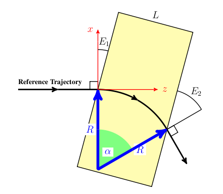
1.4.1. RBend (OPAL-t)
An RBEND is a rectangular bending magnet. The key property of an
RBEND is that it has parallel pole faces. Figure [rbend] shows an
RBEND with a positive bend angle and a positive entrance edge angle.
- L
-
Physical length of magnet (meters, see Figure [rbend]).
- GAP
-
Full vertical gap of the magnet (meters).
- HAPERT
-
Non-bend plane aperture of the magnet (meters). (Defaults to one half the bend radius.)
- ANGLE
-
Bend angle (radians). Field amplitude of bend will be adjusted to achieve this angle. (Note that for an
RBEND, the bend angle must be less than\frac{\pi}{2} + E1, whereE1is the entrance edge angle.) - K0
-
Field amplitude in y direction (Tesla). If the
ANGLEattribute is set,K0is ignored. - K0S
-
Field amplitude in x direction (Tesla). If the
ANGLEattribute is set,K0Sis ignored. - K1
-
Field gradient index of the magnet,
K_1=-\frac{R}{B_{y}}\frac{\partial B_y}{\partial x}, whereRis the bend radius as defined in Figure [rbend]. Not supported inDOPAL-tany more. Superimpose aQuadrupoleinstead. - E1
-
Entrance edge angle (radians). Figure [rbend] shows the definition of a positive entrance edge angle. (Note that the exit edge angle is fixed in an
RBENDelement to\mathrm{E2} = \mathrm{ANGLE} - \mathrm{E1}). - DESIGNENERGY
-
Energy of the reference particle (MeV). The reference particle travels approximately the path shown in Figure [rbend].
- FMAPFN
-
Name of the field map for the magnet. Currently maps of type
1DProfile1can be used see Section [1DProfile1]. The default option for this attribute isFMAPN=1DPROFILE1-DEFAULTsee Section [benddefaultfieldmapopalt]. The field map is used to describe the fringe fields of the magnet see Section [1DProfile1].
1.4.2. RBend3D (OPAL-t)
An RBEND3D3D is a rectangular bending magnet. The key property of an
RBEND3D is that it has parallel pole faces. Figure [rbend] shows an
RBEND3D with a positive bend angle and a positive entrance edge angle.
- L
-
Physical length of magnet (meters, see Figure [rbend]).
- GAP
-
Full vertical gap of the magnet (meters).
- HAPERT
-
Non-bend plane aperture of the magnet (meters). (Defaults to one half the bend radius.)
- ANGLE
-
Bend angle (radians). Field amplitude of bend will be adjusted to achieve this angle. (Note that for an
RBEND3D, the bend angle must be less than\frac{\pi}{2} + E1, whereE1is the entrance edge angle.) - K0
-
Field amplitude in y direction (Tesla). If the
ANGLEattribute is set,K0is ignored. - K0S
-
Field amplitude in x direction (Tesla). If the
ANGLEattribute is set,K0Sis ignored. - K1
-
Field gradient index of the magnet,
K_1=-\frac{R}{B_{y}}\frac{\partial B_y}{\partial x}, whereRis the bend radius as defined in Figure [rbend]. Not supported inDOPAL-tany more. Superimpose aQuadrupoleinstead. - E1
-
Entrance edge angle (radians). Figure [rbend] shows the definition of a positive entrance edge angle. (Note that the exit edge angle is fixed in an
RBEND3Delement to\mathrm{E2} = \mathrm{ANGLE} - \mathrm{E1}). - DESIGNENERGY
-
Energy of the reference particle (MeV). The reference particle travels approximately the path shown in Figure [rbend].
- FMAPFN
-
Name of the field map for the magnet. Currently maps of type
1DProfile1can be used see Section [1DProfile1]. The default option for this attribute isFMAPN=1DPROFILE1-DEFAULTsee Section [benddefaultfieldmapopalt]. The field map is used to describe the fringe fields of the magnet see Section [1DProfile1].
SBEND) with a positive bend angle \alpha. In this example the entrance and exit edge angles E_{1} and E_{2} have positive values. For a positively charge particle, the magnetic field is directed out of the page.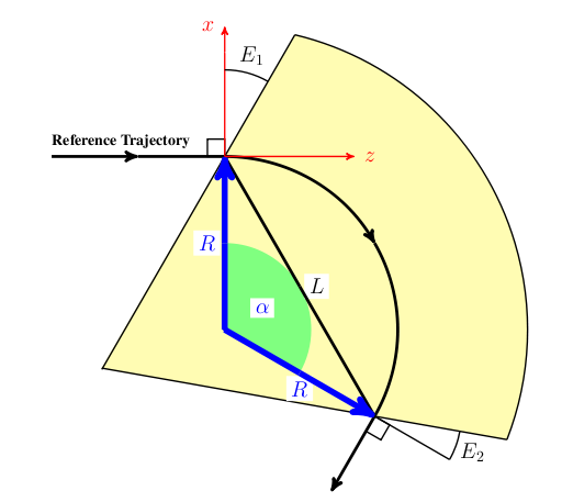
1.4.3. SBend (OPAL-t)
An SBEND is a sector bending magnet. An SBEND can have independent
entrance and exit edge angles. Figure [sbend] shows an SBEND with a
positive bend angle, a positive entrance edge angle, and a positive exit
edge angle.
- L
-
Chord length of the bend reference arc in meters (see Figure [sbend]), given by:
L = 2 R \sin\left(\frac{\alpha}{2}\right) - GAP
-
Full vertical gap of the magnet (meters).
- HAPERT
-
Non-bend plane aperture of the magnet (meters). (Defaults to one half the bend radius.)
- ANGLE
-
Bend angle (radians). Field amplitude of the bend will be adjusted to achieve this angle. (Note that practically speaking, bend angles greater than
\frac{3 \pi}{2}(270 degrees) can be problematic. Beyond this, the fringe fields from the entrance and exit pole faces could start to interfere, so be careful when setting up bend angles greater than this. An angle greater than or equal to2 \pi(360 degrees) is not allowed.) - K0
-
Field amplitude in y direction (Tesla). If the
ANGLEattribute is set,K0is ignored. - K0S
-
Field amplitude in x direction (Tesla). If the
ANGLEattribute is set,K0Sis ignored. - K1
-
Field gradient index of the magnet,
K_1=-\frac{R}{B_{y}}\frac{\partial B_y}{\partial x}, whereRis the bend radius as defined in Figure [sbend]. Not supported inDOPAL-tany more. Superimpose aQuadrupoleinstead. - E1
-
Entrance edge angle (rad). Figure [sbend] shows the definition of a positive entrance edge angle.
- E2
-
Exit edge angle (rad). Figure [sbend] shows the definition of a positive exit edge angle.
- DESIGNENERGY
-
Energy of the bend reference particle (MeV). The reference particle travels approximately the path shown in Figure [sbend].
- FMAPFN
-
Name of the field map for the magnet. Currently maps of type
1DProfile1can be used see Section [1DProfile1]. The default option for this attribute isFMAPN=1DPROFILE1-DEFAULTsee Section [benddefaultfieldmapopalt]. The field map is used to describe the fringe fields of the magnet see Section [1DProfile1].
1.4.4. RBend and SBend Examples (OPAL-t)
Describing an RBEND or an SBEND in an OPAL-t simulation requires
effectively identical commands. There are only slight differences
between the two. The L attribute has a different definition for the
two types of bends see Section [RBend,SBend], and an SBEND has an
additional attribute E2 that has no effect on an RBEND, see
Section [SBend]. Therefore, in this section, we will give several
examples of how to implement a bend, using the RBEND and SBEND
commands interchangeably. The understanding is that the command formats
are essentially the same.
When implementing an RBEND or SBEND in an OPAL-t simulation, it is
important to note the following:
-
Internally OPAL-t treats all bends as positive, as defined by Figure [rbend,sbend]. Bends in other directions within the x/y plane are accomplished by rotating a positive bend about its z axis.
-
If the
ANGLEattribute is set to a non-zero value, theK0andK0Sattributes will be ignored. -
When using the
ANGLEattribute to define a bend, the actual beam will be bent through a different angle if its mean kinetic energy doesn’t correspond to theDESIGNENERGY. -
Internally the bend geometry is setup based on the ideal reference trajectory, as shown in Figure [rbend,sbend].
-
If the default field map,
1DPROFILE-DEFAULTsee Section [benddefaultfieldmapopalt], is used, the fringe fields will be adjusted so that the effective length of the real, soft edge magnet matches the ideal, hard edge bend that is defined by the reference trajectory.
For the rest of this section, we will give several examples of how to
input bends in an OPAL-t simulation. We will start with a simple
example using the ANGLE attribute to set the bend strength and using
the default field map see Section [benddefaultfieldmapopalt] for
describing the magnet fringe fields see Section [1DProfile1]:
Bend: RBend, ANGLE = 30.0 * Pi / 180.0,
         FMAPFN = "1DPROFILE1-DEFAULT",
         ELEMEDGE = 0.25,
         DESIGNENERGY = 10.0,
         L = 0.5,
         GAP = 0.02;
This is a definition of a simple RBEND that bends the beam in a
positive direction 30 degrees (towards the negative x axis as if
Figure [rbend]). It has a design energy of 10MeV, a length of 0.5m, a
vertical gap of 2cm and a 0^{\circ} entrance edge angle.
(Therefore the exit edge angle is 30^{\circ}.) We are
using the default, internal field map "1DPROFILE1-DEFAULT"
see Section [benddefaultfieldmapopalt] which describes the magnet fringe
fields see Section [1DProfile1]. When OPAL is run, you will get the
following output (assuming an electron beam) for this RBEND
definition:
RBend > Reference Trajectory Properties
RBend > ===============================
RBend >
RBend > Bend angle magnitude:    0.523599 rad (30 degrees)
RBend > Entrance edge angle:     0 rad (0 degrees)
RBend > Exit edge angle:         0.523599 rad (30 degrees)
RBend > Bend design radius:      1 m
RBend > Bend design energy:      1e+07 eV
RBend >
RBend > Bend Field and Rotation Properties
RBend > ==================================
RBend >
RBend > Field amplitude:         -0.0350195 T
RBend > Field index (gradient):  0 m^-1
RBend > Rotation about x axis:   0 rad (0 degrees)
RBend > Rotation about y axis:   0 rad (0 degrees)
RBend > Rotation about z axis:   0 rad (0 degrees)
RBend >
RBend > Reference Trajectory Properties Through Bend Magnet with Fringe Fields
RBend > ======================================================================
RBend >
RBend > Reference particle is bent: 0.523599 rad (30 degrees) in x plane
RBend > Reference particle is bent: 0 rad (0 degrees) in y plane
The first section of this output gives the properties of the reference
trajectory like that described in Figure [rbend]. From the value of
ANGLE and the length, L, of the magnet, OPAL calculates the 10MeV
reference particle trajectory radius, R. From the bend geometry and
the entrance angle (0^{\circ} in this case), the exit
angle is calculated.
The second section gives the field amplitude of the bend and its
gradient (quadrupole focusing component), given the particle charge
(-e in this case so the amplitude is negative to get a
positive bend direction). Also listed is the rotation of the magnet
about the various axes.
Of course, in the actual simulation the particles will not see a hard
edge bend magnet, but rather a soft edge magnet with fringe fields
described by the RBEND field map file FMAPFN
see Section [1DProfile1]. So, once the hard edge bend/reference
trajectory is determined, OPAL then includes the fringe fields in the
calculation. When the user chooses to use the default field map, OPAL
will automatically adjust the position of the fringe fields
appropriately so that the soft edge magnet is equivalent to the hard
edge magnet described by the reference trajectory. To check that this
was done properly, OPAL integrates the reference particle through the
final magnet description with the fringe fields included. The result is
shown in the final part of the output. In this case we see that the soft
edge bend does indeed bend our reference particle through the correct
angle.
What is important to note from this first example, is that it is this final part of the bend output that tells you the actual bend angle of the reference particle.
In this next example, we merely rewrite the first example, but use K0
to set the field strength of the RBEND, rather than the ANGLE
attribute:
Bend: RBend, K0 = -0.0350195,
         FMAPFN = "1DPROFILE1-DEFAULT",
         ELEMEDGE = 0.25,
         DESIGNENERGY = 10.0E6,
         L = 0.5,
         GAP = 0.02;
The output from OPAL now reads as follows:
RBend > Reference Trajectory Properties
RBend > ===============================
RBend >
RBend > Bend angle magnitude:    0.523599 rad (30 degrees)
RBend > Entrance edge angle:     0 rad (0 degrees)
RBend > Exit edge angle:         0.523599 rad (30 degrees)
RBend > Bend design radius:      0.999999 m
RBend > Bend design energy:      1e+07 eV
RBend >
RBend > Bend Field and Rotation Properties
RBend > ==================================
RBend >
RBend > Field amplitude:         -0.0350195 T
RBend > Field index (gradient):  0 m^-1
RBend > Rotation about x axis:   0 rad (0 degrees)
RBend > Rotation about y axis:   0 rad (0 degrees)
RBend > Rotation about z axis:   0 rad (0 degrees)
RBend >
RBend > Reference Trajectory Properties Through Bend Magnet with Fringe Fields
RBend > ======================================================================
RBend >
RBend > Reference particle is bent: 0.5236 rad (30.0001 degrees) in x plane
RBend > Reference particle is bent: 0 rad (0 degrees) in y plane
The output is effectively identical, to within a small numerical error.
Now, let us modify this first example so that we bend instead in the negative x direction. There are several ways to do this:
1.
Bend: RBend, ANGLE = -30.0 * Pi / 180.0,
         FMAPFN = "1DPROFILE1-DEFAULT",
         ELEMEDGE = 0.25,
         DESIGNENERGY = 10.0E6,
         L = 0.5,
         GAP = 0.02;
2.
Bend: RBend, ANGLE = 30.0 * Pi / 180.0,
         FMAPFN = "1DPROFILE1-DEFAULT",
         ELEMEDGE = 0.25,
         DESIGNENERGY = 10.0E6,
         L = 0.5,
         GAP = 0.02,
         ROTATION = Pi;
3.
Bend: RBend, K0 = 0.0350195,
         FMAPFN = "1DPROFILE1-DEFAULT",
         ELEMEDGE = 0.25,
         DESIGNENERGY = 10.0E6,
         L = 0.5,
         GAP = 0.02;
4.
Bend: RBend, K0 = -0.0350195,
         FMAPFN = "1DPROFILE1-DEFAULT",
         ELEMEDGE = 0.25,
         DESIGNENERGY = 10.0E6,
         L = 0.5,
         GAP = 0.02,
         ROTATION = Pi;
In each of these cases, we get the following output for the bend (to within small numerical errors).
RBend > Reference Trajectory Properties
RBend > ===============================
RBend >
RBend > Bend angle magnitude:    0.523599 rad (30 degrees)
RBend > Entrance edge angle:     0 rad (0 degrees)
RBend > Exit edge angle:         0.523599 rad (30 degrees)
RBend > Bend design radius:      1 m
RBend > Bend design energy:      1e+07 eV
RBend >
RBend > Bend Field and Rotation Properties
RBend > ==================================
RBend >
RBend > Field amplitude:         -0.0350195 T
RBend > Field index (gradient):  -0 m^-1
RBend > Rotation about x axis:   0 rad (0 degrees)
RBend > Rotation about y axis:   0 rad (0 degrees)
RBend > Rotation about z axis:   3.14159 rad (180 degrees)
RBend >
RBend > Reference Trajectory Properties Through Bend Magnet with Fringe Fields
RBend > ======================================================================
RBend >
RBend > Reference particle is bent: -0.523599 rad (-30 degrees) in x plane
RBend > Reference particle is bent: 0 rad (0 degrees) in y plane
In general, we suggest to always define a bend in the positive x
direction (as in Figure [rbend]) and then use the ROTATION attribute
to bend in other directions in the x/y plane (as in examples 2 and 4
above).
As a final RBEND example, here is a suggested format for the four bend
definitions if one where implementing a four dipole chicane:
Bend1: RBend, ANGLE = 20.0 * Pi / 180.0,
              E1 = 0.0,
          FMAPFN = "1DPROFILE1-DEFAULT",
          ELEMEDGE = 0.25,
          DESIGNENERGY = 10.0E6,
          L = 0.25,
          GAP = 0.02,
              ROTATION = Pi;

Bend2: RBend, ANGLE = 20.0 * Pi / 180.0,
              E1 = 20.0 * Pi / 180.0,
          FMAPFN = "1DPROFILE1-DEFAULT",
          ELEMEDGE = 1.0,
          DESIGNENERGY = 10.0E6,
          L = 0.25,
          GAP = 0.02,
              ROTATION = 0.0;

Bend3: RBend, ANGLE = 20.0 * Pi / 180.0,
              E1 = 0.0,
          FMAPFN = "1DPROFILE1-DEFAULT",
          ELEMEDGE = 1.5,
          DESIGNENERGY = 10.0E6,
          L = 0.25,
          GAP = 0.02,
              ROTATION = 0.0;

Bend4: RBend, ANGLE = 20.0 * Pi / 180.0,
              E1 = 20.0 * Pi / 180.0
          FMAPFN = "1DPROFILE1-DEFAULT",
          ELEMEDGE = 2.25,
          DESIGNENERGY = 10.0E6,
          L = 0.25,
          GAP = 0.02,
              ROTATION = Pi;
Up to now, we have only given examples of RBEND definitions. If we
replaced "RBend" in the above examples with "SBend", we would still
be defining valid OPAL-t bends. In fact, by adjusting the L
attribute according to Section [RBend,SBend], and by adding the
appropriate definitions of the E2 attribute, we could even get
identical results using `SBEND`s instead of `RBEND`s. (As we said, the
two bends are very similar in command format.)
Up till now, we have only used the default field map. Custom field maps can also be used. There are two different options in this case see Section [1DProfile1]:
-
Field map defines fringe fields and magnet length.
-
Field map defines fringe fields only.
The first case describes how field maps were used in previous versions of OPAL (and can still be used in the current version). The second option is new to OPAL OPALversion1.2.00 and it has a couple of advantages:
-
Because only the fringe fields are described, the length of the magnet must be set using the
Lattribute. In turn, this means that the same field map can be used by many bend magnets with different lengths (assuming they have equivalent fringe fields). By contrast, if the magnet length is set by the field map, one must generate a new field map for each dipole of different length even if the fringe fields are the same. -
We can adjust the position of the fringe field origin relative to the entrance and exit points of the magnet see Section [1DProfile1]. This gives us another degree of freedom for describing the fringe fields, allowing us to adjust the effective length of the magnet.
We will now give examples of how to use a custom field map, starting
with the first case where the field map describes the fringe fields and
the magnet length. Assume we have the following 1DProfile1 field map:
1DProfile1 1 1 2.0
 -10.0  0.0  10.0 1
  15.0  25.0 35.0 1
  0.00000E+00
  2.00000E+00
  0.00000E+00
  2.00000E+00
We can use this field map to define the following bend (note we are now
using the SBEND command):
Bend: SBend, ANGLE = 60.0 * Pi / 180.0,
             E1 = -10.0 * Pi / 180.0,
             E2 = 20.0  Pi / 180.0,
         FMAPFN = "TEST-MAP.T7",
         ELEMEDGE = 0.25,
         DESIGNENERGY = 10.0E6,
         GAP = 0.02;
Notice that we do not set the magnet length using the L attribute.
(In fact, we don’t even include it. If we did and set it to a non-zero
value, the exit fringe fields of the magnet would not be correct.) This
input gives the following output:
SBend > Reference Trajectory Properties
SBend > ===============================
SBend >
SBend > Bend angle magnitude:    1.0472 rad (60 degrees)
SBend > Entrance edge angle:     -0.174533 rad (-10 degrees)
SBend > Exit edge angle:         0.349066 rad (20 degrees)
SBend > Bend design radius:      0.25 m
SBend > Bend design energy:      1e+07 eV
SBend >
SBend > Bend Field and Rotation Properties
SBend > ==================================
SBend >
SBend > Field amplitude:         -0.140385 T
SBend > Field index (gradient):  0 m^-1
SBend > Rotation about x axis:   0 rad (0 degrees)
SBend > Rotation about y axis:   0 rad (0 degrees)
SBend > Rotation about z axis:   0 rad (0 degrees)
SBend >
SBend > Reference Trajectory Properties Through Bend Magnet with Fringe Fields
SBend > ======================================================================
SBend >
SBend > Reference particle is bent: 1.0472 rad (60 degrees) in x plane
SBend > Reference particle is bent: 0 rad (0 degrees) in y plane
Because we set the bend strength using the ANGLE attribute, the magnet
field strength is automatically adjusted so that the reference particle
is bent exactly ANGLE radians when the fringe fields are included.
(Lower output.)
Now we will illustrate the case where the magnet length is set by the
L attribute and only the fringe fields are described by the field map.
We change the TEST-MAP.T7 file to:
1DProfile1 1 1 2.0
 -10.0  0.0  10.0 1
 -10.0  0.0  10.0 1
  0.00000E+00
  2.00000E+00
  0.00000E+00
  2.00000E+00
and change the bend input to:
Bend: SBend, ANGLE = 60.0 * Pi / 180.0,
             E1 = -10.0 * Pi / 180.0,
             E2 = 20.0  Pi / 180.0,
         FMAPFN = "TEST-MAP.T7",
         ELEMEDGE = 0.25,
         DESIGNENERGY = 10.0E6,
             L = 0.25,
         GAP = 0.02;
This results in the same output as the previous example, as we expect.
SBend > Reference Trajectory Properties
SBend > ===============================
SBend >
SBend > Bend angle magnitude:    1.0472 rad (60 degrees)
SBend > Entrance edge angle:     -0.174533 rad (-10 degrees)
SBend > Exit edge angle:         0.349066 rad (20 degrees)
SBend > Bend design radius:      0.25 m
SBend > Bend design energy:      1e+07 eV
SBend >
SBend > Bend Field and Rotation Properties
SBend > ==================================
SBend >
SBend > Field amplitude:         -0.140385 T
SBend > Field index (gradient):  0 m^-1
SBend > Rotation about x axis:   0 rad (0 degrees)
SBend > Rotation about y axis:   0 rad (0 degrees)
SBend > Rotation about z axis:   0 rad (0 degrees)
SBend >
SBend > Reference Trajectory Properties Through Bend Magnet with Fringe Fields
SBend > ======================================================================
SBend >
SBend > Reference particle is bent: 1.0472 rad (60 degrees) in x plane
SBend > Reference particle is bent: 0 rad (0 degrees) in y plane
As a final example, let us now use the previous field map with the following input:
Bend: SBend, K0 = -0.1400778,
             E1 = -10.0 * Pi / 180.0,
             E2 = 20.0  Pi / 180.0,
         FMAPFN = "TEST-MAP.T7",
         ELEMEDGE = 0.25,
         DESIGNENERGY = 10.0E6,
             L = 0.25,
         GAP = 0.02;
Instead of setting the bend strength using ANGLE, we use K0. This
results in the following output:
SBend > Reference Trajectory Properties
SBend > ===============================
SBend >
SBend > Bend angle magnitude:    1.0472 rad (60 degrees)
SBend > Entrance edge angle:     -0.174533 rad (-10 degrees)
SBend > Exit edge angle:         0.349066 rad (20 degrees)
SBend > Bend design radius:      0.25 m
SBend > Bend design energy:      1e+07 eV
SBend >
SBend > Bend Field and Rotation Properties
SBend > ==================================
SBend >
SBend > Field amplitude:         -0.140078 T
SBend > Field index (gradient):  0 m^-1
SBend > Rotation about x axis:   0 rad (0 degrees)
SBend > Rotation about y axis:   0 rad (0 degrees)
SBend > Rotation about z axis:   0 rad (0 degrees)
SBend >
SBend > Reference Trajectory Properties Through Bend Magnet with Fringe Fields
SBend > ======================================================================
SBend >
SBend > Reference particle is bent: 1.04491 rad (59.8688 degrees) in x plane
SBend > Reference particle is bent: 0 rad (0 degrees) in y plane
In this case, the bend angle for the reference trajectory in the first section of the output no longer matches the reference trajectory bend angle from the lower section (although the difference is small). The reason is that the path of the reference particle through the real magnet (with fringe fields) no longer matches the ideal trajectory. (The effective length of the real magnet is not quite the same as the hard edged magnet for the reference trajectory.)
We can compensate for this by changing the field map file TEST-MAP.T7 file to:
1DProfile1 1 1 2.0
 -10.0  -0.03026  10.0 1
 -10.0  0.03026  10.0 1
  0.00000E+00
  2.00000E+00
  0.00000E+00
  2.00000E+00
We have moved the Enge function origins see Section [1DProfile1] outward from the entrance and exit faces of the magnet see Section [1DProfile1] by 0.3026 mm. This has the effect of making the effective length of the soft edge magnet longer. When we do this, the same input:
Bend: SBend, K0 = -0.1400778,
             E1 = -10.0 * Pi / 180.0,
             E2 = 20.0  Pi / 180.0,
         FMAPFN = "TEST-MAP.T7",
         ELEMEDGE = 0.25,
         DESIGNENERGY = 10.0E6,
             L = 0.25,
         GAP = 0.02;
produces
SBend > Reference Trajectory Properties
SBend > ===============================
SBend >
SBend > Bend angle magnitude:    1.0472 rad (60 degrees)
SBend > Entrance edge angle:     -0.174533 rad (-10 degrees)
SBend > Exit edge angle:         0.349066 rad (20 degrees)
SBend > Bend design radius:      0.25 m
SBend > Bend design energy:      1e+07 eV
SBend >
SBend > Bend Field and Rotation Properties
SBend > ==================================
SBend >
SBend > Field amplitude:         -0.140078 T
SBend > Field index (gradient):  0 m^-1
SBend > Rotation about x axis:   0 rad (0 degrees)
SBend > Rotation about y axis:   0 rad (0 degrees)
SBend > Rotation about z axis:   0 rad (0 degrees)
SBend >
SBend > Reference Trajectory Properties Through Bend Magnet with Fringe Fields
SBend > ======================================================================
SBend >
SBend > Reference particle is bent: 1.0472 rad (60 degrees) in x plane
SBend > Reference particle is bent: 0 rad (0 degrees) in y plane
Now we see that the bend angle for the ideal, hard edge magnet, matches the bend angle of the reference particle through the soft edge magnet. In other words, the effective length of the soft edge, real magnet is the same as the hard edge magnet described by the reference trajectory.
1.4.5. Bend Fields from 1D Field Maps (OPAL-t)
1DProfile1 field map described in Section [benddefaultfieldmapopalt]. The exit fringe field of this magnet is the mirror image.
So far we have described how to setup an RBEND or SBEND element, but
have not explained how OPAL-t uses this information to calculate the
magnetic field. The field of both types of magnets is divided into three
regions:
-
Entrance fringe field.
-
Central field.
-
Exit fringe field.
This can be seen clearly in Figure [rbend_field_profile].
The purpose of the 1DProfile1 field map see Section [1DProfile1]
associated with the element is to define the Enge functions
(Equation [enge_func]) that model the entrance and exit fringe fields.
To model a particular bend magnet, one must fit the field profile along
the mid-plane of the magnet perpendicular to its face for the entrance
and exit fringe fields to the Enge function:
F(z) = \frac{1}{1 + e^{\sum\limits_{n=0}^{N_{order}} c_{n} (z/D)^{n}}}where D is the full gap of the magnet,
N_{order} is the Enge function order and z
is the distance from the origin of the Enge function perpendicular to
the edge of the dipole. The origin of the Enge function, the order of
the Enge function, N_{order}, and the constants
c_0 to c_{N_{order}} are free parameters
that are chosen so that the function closely approximates the fringe
region of the magnet being modeled. An example of the entrance fringe
field is shown in Figure [rbend_enge_fringe].
Let us assume we have a correctly defined positive RBEND or SBEND
element as illustrated in Figure [rbend,sbend]. (As already stated, any
bend can be described by a rotated positive bend.) OPAL-t then has the
following information:
\begin{aligned}
B_0 &= \text{Field amplitude (T)} \\
R &= \text{Bend radius (m)} \\
n &= -\frac{R}{B_{y}}\frac{\partial B_y}{\partial x} \text{ (Field index, set using the parameter } \mathrm{K1} \text{)} \\
F(z) &= \left\{
\begin{array}{lll}
    & F_{entrance}(z_{entrance}) \\
    & F_{center}(z_{center}) = 1 \\
    & F_{exit}(z_{exit})
\end{array}
\right.\end{aligned}
Here, we have defined an overall Enge function, F(z), with
three parts: entrance, center and exit. The exit and entrance fringe
field regions have the form of Equation [enge_func] with parameters
defined by the 1DProfile1 field map file given by the element
parameter FMAPFN. Defining the coordinates:
\begin{aligned}
y &\equiv \text{Vertical distance from magnet mid-plane} \\
\Delta_x &\equiv \text{Perpendicular distance to reference trajectory (see Figures)} \\
\Delta_z &\equiv \left\{
\begin{array}{lll}
    & \text{Distance from entrance Enge function origin perpendicular to magnet entrance face.} \\
    & \text{Not defined, Enge function is always 1 in this region.} \\
    & \text{Distance from exit Enge function origin perpendicular to magnet exit face.}
\end{array}
\right.\end{aligned}
using the conditions
\begin{aligned}
\nabla \cdot \vec{B} &= 0 \\
\nabla \times \vec{B} &= 0
\end{aligned}
and making the definitions:
\begin{aligned}
F'(z) &\equiv   \frac{\mathrm{d} F(z)}{\mathrm{d} z} \\
F''(z) &\equiv  \frac{\mathrm{d^{2}} F(z)}{\mathrm{d} z^{2}} \\
F'''(z) &\equiv \frac{\mathrm{d^{3}} F(z)}{\mathrm{d} z^{3}}
\end{aligned}
we can expand the field off axis, with the result:
\begin{aligned}
B_x(\Delta_x, y, \Delta_z) &= -\frac{B_0 \frac{n}{R}}{\sqrt{\frac{n^2}{R^2} +  \frac{F''(\Delta_z)}{F(\Delta_z}}} e^{-\frac{n}{R} \Delta_x} \sin \left[ \left( \sqrt{\frac{n^2}{R^2} + \frac{F''(\Delta_z)}{F(\Delta_z)}} \right) y \right] F(\Delta_z) \\
B_y(\Delta_x, y, \Delta_z) &= B_0 e^{-\frac{n}{R} \Delta_x} \cos \left[ \left( \sqrt{\frac{n^2}{R^2} + \frac{F''(\Delta_z)}{F(\Delta_z)}} \right) y \right] F(\Delta_z) \\
B_z(\Delta_x, y, \Delta_z) &= B_0 e^{-\frac{n}{R} \Delta_x} \left\{\frac{F'(\Delta_z)}{\sqrt{\frac{n^2}{R^2} + \frac{F''(\Delta_z)}{F(\Delta_z)}}} \sin \left[ \left( \sqrt{\frac{n^2}{R^2} + \frac{F''(\Delta_z)}{F(\Delta_z)}} \right) y \right] \right. \\
&- \frac{1}{2 \sqrt{\frac{n^2}{R^2} + \frac{F''(\Delta_z)}{F(\Delta_z)}}} \left(F'''(\Delta_z) - \frac{F'(\Delta_z) F''(\Delta_z)}{F(\Delta_z)} \right) \left[ \frac{\sin \left[ \left( \sqrt{\frac{n^2}{R^2} + \frac{F''(\Delta_z)}{F(\Delta_z)}} \right) y \right]}{\frac{n^2}{R^2} + \frac{F''(\Delta_z)}{F(\Delta_z)}} \right. \\
&- \left. \left. y \frac{\cos \left[ \left( \sqrt{\frac{n^2}{R^2} + \frac{F''(\Delta_z)}{F(\Delta_z)}} \right) y \right]}{\sqrt{\frac{n^2}{R^2} + \frac{F''(\Delta_z)}{F(\Delta_z)}}} \right] \right\}\end{aligned}
These expression are not well suited for numerical calculation, so, we
expand them about y to O(y^2) to obtain:
-
In fringe field regions:
\begin{aligned}
B_x(\Delta_x, y, \Delta_z) &\approx -B_0 \frac{n}{R} e^{-\frac{n}{R} \Delta_x} y \\
B_y(\Delta_x, y, \Delta_z) &\approx B_0 e^{-\frac{n}{R} \Delta_x} \left[ F(\Delta_z) - \left( \frac{n^2}{R^2} F(\Delta_z) + F''(\Delta_z) \right) \frac{y^2}{2} \right] \\
B_z(\Delta_x, y, \Delta_z) &\approx B_0 e^{-\frac{n}{R} \Delta_x} y F'(\Delta_z)
\end{aligned}-
In central region:
\begin{aligned}
B_x(\Delta_x, y, \Delta_z) &\approx -B_0 \frac{n}{R} e^{-\frac{n}{R} \Delta_x} y \\
B_y(\Delta_x, y, \Delta_z) &\approx B_0 e^{-\frac{n}{R} \Delta_x} \left[ 1 -  \frac{n^2}{R^2} \frac{y^2}{2} \right] \\
B_z(\Delta_x, y, \Delta_z) &\approx 0
\end{aligned}
These are the expressions OPAL-t uses to calculate the field inside an
RBEND or SBEND. First, a particle’s position inside the bend is
determined (entrance region, center region, or exit region). Depending
on the region, OPAL-t then determines the values of
\Delta_x, y and \Delta_z, and
then calculates the field values using the above expressions.
1.4.6. Default Field Map (OPAL-t)
Rather than force users to calculate the field of a dipole and then fit
that field to find Enge coefficients for the dipoles in their
simulation, we have a default set of values we use from [enge] that are
set when the default field map, 1DPROFILE1-DEFAULT is used:
\begin{aligned}
  c_{0} &= 0.478959 \\
  c_{1} &= 1.911289 \\
  c_{2} &= -1.185953 \\
  c_{3} &= 1.630554 \\
  c_{4} &= -1.082657 \\
  c_{5} &= 0.318111\end{aligned}
The same values are used for both the entrance and exit regions of the magnet. In general they will give good results. (Of course, at some point as a beam line design becomes more advanced, one will want to find Enge coefficients that fit the actual magnets that will be used in a given design.)
The default field map is the equivalent of the following custom
1DProfile1 (see Section [1DProfile1] for an explanation of the field
map format) map:
1DProfile1 5 5 2.0
 -10.0 0.0 10.0 1
 -10.0 0.0 10.0 1
  0.478959
  1.911289
 -1.185953
  1.630554
 -1.082657
  0.318111
  0.478959
  1.911289
 -1.185953
  1.630554
 -1.082657
  0.318111
As one can see, the default magnet gap for 1DPROFILE1-DEFAULT is
set to 2.0cm. This value can be overridden by the GAP attribute of the
magnet (see Section [RBend,SBend]).
1.4.7. SBend3D (OPAL-CYCL)
The SBend3D element enables definition of a bend from 3D field maps.
This can be used in conjunction with the RINGDEFINITION element to
make a ring for tracking through OPAL-cycl.
label: SBEND3D, FMAPFN=string, LENGTH_UNITS=real, FIELD_UNITS=real;
- FMAPFN
-
The field map file name.
- LENGTH_UNITS
-
Units for length (set to 1.0 for units in mm, 10.0 for units in cm, etc).
- FIELD_UNITS
-
Units for field (set to 1.0 for units in T, 0.001 for units in mT, etc).
Field maps are defined using Cartesian coordinates but in a polar geometry with the following restrictions/conventions:
-
3D Field maps have to be generated in the vertical direction (z coordinate in OPAL-cycl) from z = 0 upwards. It cannot be generated symmetrically about z = 0 towards negative z values.
-
Field map file must be in the form with columns ordered as follows: [
x, z, y, B_{x}, B_{z}, B_{y}]. -
Grid points of the position and field strength have to be written on a grid in (
r, z, \theta) with the primary direction corresponding to the azimuthal direction, secondary to the vertical direction and tertiary to the radial direction.
Below two examples of a SBEND3D which loads a field maps with
different units. The triplet example has units of cm and fields units
of Gauss, where the Dipole example (Figure [sbend3d1]) uses meter and
Tesla. The first 8 lines in the field map are ignored.
triplet: SBEND3D, FMAPFN="fdf-tosca-field-map.table", LENGTH_UNITS=10., FIELD_UNITS=-1e-4;
The first few links of the field map fdf-tosca-field-map.table:
      422280      422280      422280           1
 1 X [LENGU]
 2 Y [LENGU]
 3 Z [LENGU]
 4 BX [FLUXU]
 5 BY [FLUXU]
 6 BZ [FLUXU]
 0
 194.01470 0.0000000 80.363520 0.68275932346E-07 -5.3752492577 0.28280706805E-07
 194.36351 0.0000000 79.516210 0.42525693524E-07 -5.3827955117 0.17681348191E-07
 194.70861 0.0000000 78.667380 0.19766168358E-07 -5.4350026348 0.82540823165E-08
.....
Dipole:SBEND3D,FMAPFN="90degree_Dipole_Magnet.out",LENGTH_UNITS=1000.0, FIELD_UNITS=-10.0;
The first few links of the field map 90degree_Dipole_Magnet.out:
    4550000 4550000 4550000 1
X [LENGTH_UNITS]
Z [LENGTH_UNITS]
Y [LENGTH_UNITS]
BX [FIELD_UNITS]
BZ [FIELD_UNITS]
BY [FIELD_UNITS]
0
4.3586435e-01   5.0000000e-02   1.2803431e+00   0.0000000e+00   1.6214000e+00   0.0000000e+00
4.2691532e-01   5.0000000e-02   1.2833548e+00   0.0000000e+00   1.6214000e+00   0.0000000e+00
4.1794548e-01   5.0000000e-02   1.2863039e+00   0.0000000e+00   1.6214000e+00   0.0000000e+00
...
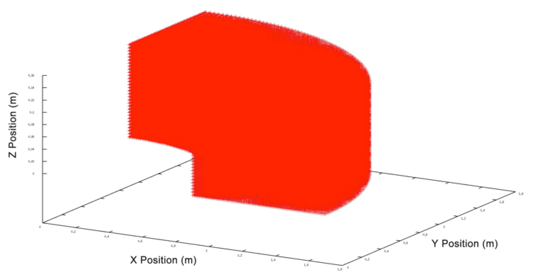
This is a restricted feature: OPAL-cycl.
90 degree dipole magnet with homogeneous magnetic field. The right figure is showing the horizontal cross section of the 3D magnetic field map when z = 0

1.5. Quadrupole
label:QUADRUPOLE, TYPE=string, APERTURE=real-vector,
      L=real, K1=real, K1S=real;
The reference system for a quadrupole is a Cartesian coordinate system
This is a restricted feature: DOPAL-cycl.
A QUADRUPOLE has three real attributes:
- K1
-
The normal quadrupole component
K_1=\frac{\partial B_y}{\partial x}. The default is0 Tm^{-1}. The component is positive, ifB_yis positive on the positivex-axis. This implies horizontal focusing of positively charged particles which travel in positives-direction. - K1S
-
The skew quadrupole component.
K_{1s}=-\frac{\partial B_x}{\partial x}. The default is0 Tm^{-1}. The component is negative, ifB_xis positive on the positivex-axis.
Example:
QP1: Quadrupole, L=1.20, ELEMEDGE=-0.5265,
     FMAPFN="1T1.T7", K1=0.11;
1.6. Sextupole
label: SEXTUPOLE, TYPE=string, APERTURE=real-vector,
       L=real, K2=real, K2S=real;
A SEXTUPOLE has three real attributes:
- K2
-
The normal sextupole component
K_2=\frac{\partial{^2} B_y}{\partial x^2}. The default is{0}{T m^{-2}}. The component is positive, ifB_yis positive on thex-axis. - K2S
-
The skew sextupole component
K_{2s}=-\frac{\partial{^2}B_x}{\partial x^{2}}. The default is{0}{T m^{-2}}. The component is negative, ifB_xis positive on thex-axis.
Example:
S:SEXTUPOLE, L=0.4, K2=0.00134;
The reference system for a sextupole is a Cartesian coordinate system
1.7. Octupole
label:OCTUPOLE, TYPE=string, APERTURE=real-vector,
      L=real, K3=real, K3S=real;
An OCTUPOLE has three real attributes:
- K3
-
The normal octupole component
K_3=\frac{\partial{^3} B_y}{\partial x^3}. The default is{0}{Tm^{-3}}. The component is positive, ifB_yis positive on the positivex-axis. - K3S
-
The skew octupole component
K_{3s}=-\frac{\partial{^3}B_x}{\partial x^{3}}. The default is{0}{Tm^{-3}}. The component is negative, ifB_xis positive on the positivex-axis.
Example:
O3:OCTUPOLE, L=0.3, K3=0.543;
The reference system for an octupole is a Cartesian coordinate system
1.8. General Multipole
A MULTIPOLE is in OPAL-t is of arbitrary order.
label:MULTIPOLE, TYPE=string, APERTURE=real-vector,
      L=real, KN=real-vector, KS=real-vector;
- KN
-
A real vector see Section [anarray], containing the normal multipole coefficients,
K_n=\frac{\partial{^n} B_y}{\partial x^n}. (default is{0}{Tm^{-n}}). A component is positive, ifB_yis positive on the positivex-axis. - KS
-
A real vector see Section [anarray], containing the skew multipole coefficients,
K_{n~s}=-\frac{\partial{^n}B_x}{\partial x^{n}}. (default is{0}{Tm^{-n}}). A component is negative, ifB_xis positive on the positivex-axis.
The order n is unlimited, but all components up to the
maximum must be given, even if they are zero. The number of poles of
each component is (2 n + 2).
Superposition of many multipole components is permitted. The reference system for a multipole is a Cartesian coordinate system
The following example is equivalent to the quadruple example in Section [quadrupole].
M27:MULTIPOLE, L=1, ELEMEDGE=3.8, KN={0.0,0.11};
A multipole has no effect on the reference orbit, i.e. the reference system at its exit is the same as at its entrance. Use the dipole component only to model a defective multipole.
1.9. General Multipole (will replace Section [multipole] when implemented)
A MULTIPOLET is in OPAL-t a general multipole with extended
features. It can represent a straight or curved magnet. In the curved
case, the user may choose between constant or variable radius. This
model includes fringe fields. The detailed description can be found at:
https://gitlab.psi.ch/OPAL/src/uploads/0d3fc561b57e8962ed79a57cd6115e37/8FBB32A4-7FA1-4084-A4A7-CDDB1F949CD3_psi.ch.pdf.
label:MULTIPOLET, L=real, ANGLE=real, VAPERT=real, HAPERT=real,
      LFRINGE=real, RFRINGE=real, TP=real-vector, VARRADIUS=bool;
- L
-
Physical length of the magnet (meters), without end fields. (Default: 1 m)
- ANGLE
-
Physical angle of the magnet (radians). If not specified, the magnet is considered to be straight (ANGLE=0.0). This is not the total bending angle since the end fields cause additional bending. The radius of the multipole is set from the LENGTH and ANGLE attributes.
- VAPERT
-
Vertical (non-bend plane) aperture of the magnet (meters). (Default: 0.5 m)
- HAPERT
-
Horizontal (bend plane) aperture of the magnet (meters). (Default: 0.5 m)
- LFRINGE
-
Length of the left fringe field (meters). (Default: 0.0 m)
- RFRINGE
-
Length of the right fringe field (meters). (Default: 0.0 m)
- TP
-
A real vector see Section [anarray], containing the multipole coefficients of the field expansion on the mid-plane in the body of the magnet: the transverse profile
T(x) = B_0 + B_1 x + B_2 x^2 + \ldotsis set by TP=B_0,B_1,B_2(units:T \cdot m^{-n}). The order of highest multipole component is arbitrary, but all components up to the maximum must be given, even if they are zero. - MAXFORDER
-
The order of the maximum function
f_nused in the field expansion (default: 5). See the scalar magnetic potential below. This sets for example the maximum power ofzin the field expansion of vertical componentB_zto2 \cdot \text{MAXFORDER}. - EANGLE
-
Entrance edge angle (radians).
- ROTATION
-
Rotation of the magnet about its central axis (radians, counterclockwise). This enables to obtain skew fields. (Default 0.0 rad)
- VARRADIUS
-
This is to be set TRUE if the magnet has variable radius. More precisely, at each point along the magnet, its radius is computed such that the reference trajectory always remains in the centre of the magnet. In the body of the magnet the radius is set from the LENGTH and ANGLE attributes. It is then continuously changed to be proportional to the dipole field on the reference trajectory while entering the end fields. This attribute is only to be set TRUE for a non-zero dipole component. (Default: FALSE)
- VARSTEP
-
The step size (meters) used in calculating the reference trajectory for VARRARDIUS = TRUE. It specifies how often the radius of curvature is re-calculated. This has a considerable effect on tracking time. (Default: 0.1 m)
Superposition of many multipole components is permitted. The reference
system for a multipole is a Cartesian coordinate system for straight
geometry and a (x,s,z) Frenet-Serret coordinate system for
curved geometry. In the latter case, the axis \hat{s} is
the central axis of the magnet.
1.10. Solenoid
label:SOLENOID, TYPE=string, APERTURE=real-vector,
      L=real, KS=real;
A SOLENOID has two real attributes:
- KS
-
The solenoid strength
K_s=\frac{\partial B_s}{\partial s}, default is{0}{Tm^{-1}}. For positiveKSand positive particle charge, the solenoid field points in the direction of increasings.
The reference system for a solenoid is a Cartesian coordinate system Using a solenoid in OPAL-t mode, the following additional parameters are defined:
- FMAPFN
-
Field maps must be specified.
Example:
SP1: Solenoid, L=1.20, ELEMEDGE=-0.5265, KS=0.11,
     FMAPFN="1T1.T7";
1.11. Cyclotron
label:CYCLOTRON, TYPE=string, CYHARMON=int,
      PHIINIT=real, PRINIT=real, RINIT=real,
      SYMMETRY=real, RFFREQ=real, FMAPFN=string;
A CYCLOTRON object includes the main characteristics of a cyclotron,
the magnetic field, and also the initial condition of the injected
reference particle, and it has currently the following attributes:
- TYPE
-
The data format of field map, Currently three formats are implemented: CARBONCYCL, CYCIAE, AVFEQ, FFAG, BANDRF and default PSI format. For the details of their data format, please read Section [opalcycl:fieldmap].
- CYHARMON
-
The harmonic number of the cyclotron
h. - RFFREQ
-
The RF system
f_{rf}(unit:MHz, default: 0). The particle revolution frequencyf_{rev}=f_{rf}/h. - FMAPFN
-
File name for the magnetic field map.
- SYMMETRY
-
Defines symmetrical fold number of the B field map data.
- RINIT
-
The initial radius of the reference particle (unit: mm, default: 0)
- PHIINIT
-
The initial azimuth of the reference particle (unit: degree, default: 0)
- ZINIT
-
The initial axial position of the reference particle (unit: mm, default: 0)
- PRINIT
-
Initial radial momentum of the reference particle
P_r=\beta_r\gamma(default : 0) - PZINIT
-
Initial axial momentum of the reference particle
P_z=\beta_z\gamma(default : 0) - MINZ
-
The minimal vertical extent of the machine (unit: mm, default : -10000.0)
- MAXZ
-
The maximal vertical extent of the machine (unit: mm, default : 10000.0)
- MINR
-
Minimal radial extent of the machine (unit: mm, default : 0.0)
- MAXR
-
Minimal radial extent of the machine (unit: mm, default : 10000.0)
During the tracking, the particle (r, z, \theta) will be
deleted if MINZ < z < MAXZ or MINR < r <
MAXR, and it will be recorded in the ASCII file <inputfilename>.loss.
Example:
ring: Cyclotron, TYPE="RING", CYHARMON=6, PHIINIT=0.0,
      PRINIT=-0.000240, RINIT=2131.4 , SYMMETRY=8.0,
      RFFREQ=50.650, FMAPFN="s03av.nar",
      MAXZ=10, MINZ=-10, MINR=0, MAXR=2500;
If TYPE is set to BANDRF, the 3D electric field map of RF cavity will be read from external h5part file and 4 extra arguments need to specified:
- RFMAPFN
-
The file name for the electric field map in h5part binary format.
- RFPHI
-
The Initial phase of the electric field map (rad)
- ESCALE
-
The maximal value of the electric field map (MV/m)
- SUPERPOSE
-
An option whether all of the electric field maps are superposed, The is valid when more than one electric field map is read. (default: true)
Example for single electric field map:
COMET: Cyclotron, TYPE="BANDRF", CYHARMON=2, PHIINIT= -71.0,
PRINIT=pr0, RINIT= r0 , SYMMETRY=1.0, FMAPFN="Tosca_map.txt",
RFPHI=Pi, RFFREQ=72.0,  RFMAPFN="efield.h5part",
ESCALE=1.06E-6;
We can have more than one RF field maps.
Example for multiple RF field maps:
COMET: Cyclotron, TYPE="BANDRF", CYHARMON=2, PHIINIT=-71.0,
PRINIT=pr0, RINIT=r0 , SYMMETRY=1.0, FMAPFN="Tosca_map.txt",
RFPHI= {Pi,0,Pi,0}, RFFREQ={72.0,72.0,72.0,72.0},
RFMAPFN={"e1.h5part","e2.h5part","e3.h5part","e4.h5part"},
ESCALE={1.06E-6, 3.96E-6,1.3E-6,1.E-6}, SUPERPOSE=true;
In this example SUPERPOSE is set to true. Therefore, if a particle locates in multiple field regions, all the field maps are superposed. if SUPERPOSE is set to false, then only one field map, which has highest priority, is used to do interpolation for the particle tracking. The priority ranking is decided by their sequence in the list of RFMAPFN argument, i.e., "e1.h5hart" has the highest priority and "e4.h5hart" has the lowest priority.
Another method to model an RF cavity is to read the RF voltage profile in the RFCAVITY element see Section [cavity] and make a momentum kick when a particle crosses the RF gap. In the center region of the compact cyclotron, the electric field shape is complicated and may make a significant impact on transverse beam dynamics. Hence a simple momentum kick is not enough and we need to read 3D field map to do precise simulation.
In addition, the simplified trim-coil field model is also implemented so as to do fine tuning on the magnetic field. A trim-coil can be defined by 4 arguments:
- TCR1
-
Array of inner radii of the trim coils (mm)
- TCR2
-
Array of outer radii of the trim coils (mm)
- MBTC
-
Array of the maximal B field of the trim coils (kG)
- SLPTC
-
Array of the slopes of the rising edge (1/mm)
This is a restricted feature: OPAL-cycl.
1.12. Ring Definition
label: RINGDEFINITION,
       RFFREQ=real, HARMONIC_NUMBER=real, IS_CLOSED=string, SYMMETRY=int,
       LAT_RINIT=real, LAT_PHIINIT=real, LAT_THETAINIT=real,
       BEAM_PHIINIT=real, BEAM_PRINIT=real, BEAM_RINIT=real;
A RingDefinition object contains the main characteristics of a
generalized ring. The RingDefinition lists characteristics of the
entire ring such as harmonic number together with the position of the
initial element and the position of the reference trajectory.
The RingDefinition can be used in combination with SBEND3D, offsets
and VARIABLE_RF_CAVITY elements to make up a complete ring.
- RFFREQ
-
Nominal RF frequency of the ring [MHz].
- HARMONIC_NUMBER
-
The harmonic number of the ring - i.e. number of bunches in a single pass.
- SYMMETRY
-
Azimuthal symmetry of the ring. Ring elements will be placed repeatedly
SYMMETRYtimes. - IS_CLOSED
-
Set to
FALSEto disable checking for ring closure. - LAT_RINIT
-
Radius of the first element placement in the lattice [mm].
- LAT_PHIINIT
-
Azimuthal angle of the first element placed in the lattice [degree].
- LAT_THETAINIT
-
Angle in the mid-plane relative to the ring tangent for placement of the first element [degree].
- BEAM_RINIT
-
Initial radius of the reference trajectory [mm].
- BEAM_PHIINIT
-
Initial azimuthal angle of the reference trajectory [degree].
- BEAM_PRINIT
-
Transverse momentum
\beta \gammafor the reference trajectory.
In the following example, we define a ring with radius 2.35 m and 4 cells.
ringdef: RINGDEFINITION, HARMONIC_NUMBER=6, LAT_RINIT=2350.0, LAT_PHIINIT=0.0,
         LAT_THETAINIT=0.0, BEAM_PHIINIT=0.0, BEAM_PRINIT=0.0,
         BEAM_RINIT=2266.0, SYMMETRY=4.0, RFFREQ=0.2;
1.12.1. Local Cartesian Offset
The LOCAL_CARTESIAN_OFFSET enables the user to place an object at an
arbitrary position in the coordinate system of the preceding element.
This enables drift spaces and placement of overlapping elements.
- END_POSITION_X
-
x position of the next element start in the coordinate system of the preceding element [mm].
- END_POSITION_Y
-
y position of the next element start in the coordinate system of the preceding element [mm].
- END_NORMAL_X
-
x component of the normal vector defining the placement of the next element in the coordinate system of the preceding element.
- END_NORMAL_Y
-
y component of the normal vector defining the placement of the next element in the coordinate system of the preceding element.
1.13. Source
This element only works in OPAL-t. It’s only purpose in OPAL-t is to
indicate that the particle source is contained in the beamline. This is
needed to place the elements in three-dimensional space when using
ELEMEDGE. Otherwise it has no effect on the particles.
1.14. RF Cavities (OPAL-t and OPAL-cycl)
For an RFCAVITY the three modes have four real attributes in common:
label:RFCAVITY, APERTURE=real-vector, L=real,
      VOLT=real, LAG=real;
- L
-
The length of the cavity (default: 0 m)
- VOLT
-
The peak RF voltage (default: 0 MV). The effect of the cavity is
\delta E=\mathrm{VOLT}\cdot\sin(2\pi(\mathrm{LAG}-\mathrm{HARMON}\cdot f_0 t)). - LAG
-
The phase lag [rad] (default: 0). In OPAL-t this phase is in general relative to the phase at which the reference particle gains the most energy. This phase is determined using an auto-phasing algorithm (see Appendix [autophasing]). This auto-phasing algorithm can be switched off, see
APVETO.
1.14.1. OPAL-t mode
Using a RF Cavity in OPAL-t mode, the following additional parameters are defined:
- FMAPFN
-
Field maps in the T7 format can be specified.
- TYPE
-
Type specifies STANDING [default] or SINGLE GAP structures.
- FREQ
-
Defines the frequency of the RF Cavity in units of MHz. A warning is issued when the frequency of the cavity card does not correspond to the frequency defined in the FMAPFN file. The frequency of the cavity card overrides the frequency defined in the FMAPFN file.
- APVETO
-
If
TRUEthis cavity will not be auto-phased. Instead the phase of the cavity is equal toLAGat the arrival time of the reference particle (arrival at the limit of its field not atELEMEDGE).
Example standing wave cavity which mimics a DC gun:
gun: RFCavity, L=0.018, VOLT=-131/(1.052*2.658),
     FMAPFN="1T3.T7", ELEMEDGE=0.00,
     TYPE="STANDING", FREQ=1.0e-6;
Example of a two frequency standing wave cavity:
rf1: RFCavity, L=0.54, VOLT=19.961, LAG=193.0/360.0,
     FMAPFN="1T3.T7", ELEMEDGE=0.129, TYPE="STANDING",
     FREQ=1498.956;
rf2: RFCavity, L=0.54, VOLT=6.250, LAG=136.0/360.0,
     FMAPFN="1T4.T7", ELEMEDGE=0.129, TYPE="STANDING",
     FREQ=4497.536;
1.14.2. OPAL-cycl mode
Using a RF Cavity (standing wave) in OPAL-cycl mode, the following parameters are defined:
- FMAPFN
-
Defines name of file which stores normalized voltage amplitude curve of cavity gap in ASCII format. (See data format in Section [opalcycl:rffieldmap])
- VOLT
-
Sets peak value of voltage amplitude curve in MV.
- TYPE
-
Defines Cavity type, SINGLEGAP represents cyclotron type cavity.
- FREQ
-
Sets the frequency of the RF Cavity in units of MHz.
- RMIN
-
Sets the radius of the cavity inner edge in mm.
- RMAX
-
Sets the radius of the cavity outer edge in mm.
- ANGLE
-
Sets the azimuthal position of the cavity in global frame in degree.
- PDIS
-
Set shift distance of cavity gap from center of cyclotron in mm. If its value is positive, the shift direction is clockwise, namely, shift towards the smaller azimuthal angle.
- GAPWIDTH
-
Set gap width of cavity in mm.
- PHI0
-
Set initial phase of cavity in degree.
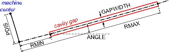
Example of a RF cavity of cyclotron:
rf0: RFCavity, VOLT=0.25796, FMAPFN="Cav1.dat",
     TYPE="SINGLEGAP", FREQ=50.637, RMIN = 350.0,
     RMAX = 3350.0, ANGLE=35.0,   PDIS = 0.0,
     GAPWIDTH = 0.0, PHI0=phi01;
Figure [Cyclotron_cavity] shows the simplified geometry of a cavity gap and its parameters.
1.15. RF Cavities with Time Dependent Parameters
The VARIABLE_RF_CAVITY element can be used to define RF Cavities with
Time Dependent Parameters in OPAL-cycl mode. Variable RF Cavities must
be placed using the RingDefinition element.
- FREQUENCY_MODEL
-
String naming the time dependence model of the cavity frequency,
f[MHz]. - AMPLITUDE_MODEL
-
String naming the time dependence model of the cavity amplitude,
E_0[MV/m]. - PHASE_MODEL
-
String naming the time dependence model of the cavity phase offset,
\phi. - WIDTH
-
Full width of the cavity [mm].
- HEIGHT
-
Full height of the cavity [mm].
- L
-
Full length of the cavity [mm].
The field inside the cavity is given by
\mathbf{E} = \big(0, 0, E_0(t)\sin[2\pi f(t) t+\phi(t)]\big)with no field outside the cavity boundary. There is no magnetic field or transverse dependence on electric field.
1.15.1. Time Dependence
The POLYNOMIAL_TIME_DEPENDENCE element is used to define time
dependent parameters in RF cavities in terms of a third order
polynomial.
- P0
-
Constant term in the polynomial expansion.
- P1
-
First order term in the polynomial expansion [ns
^{-1}]. - P2
-
Second order term in the polynomial expansion [ns
^{-2}]. - P3
-
Third order term in the polynomial expansion [ns
^{-3}].
The polynomial is evaluated as
g(t) = p_0 + p_1 t + p_2 t^2 + p_3 t^3.An example of a Variable Frequency RF cavity of cyclotron with polynomial time dependence of parameters is given below:
REAL phi=2.*PI*0.25;

REAL rf_p0=0.00158279;
REAL rf_p1=9.02542e-10;
REAL rf_p2=-1.96663e-16;
REAL rf_p3=2.45909e-23;

RF_FREQUENCY: POLYNOMIAL_TIME_DEPENDENCE, P0=rf_p0, P1=rf_p1, P2=rf_p2, P3=rf_p3;
RF_AMPLITUDE: POLYNOMIAL_TIME_DEPENDENCE, P0=1.0;
RF_PHASE: POLYNOMIAL_TIME_DEPENDENCE, P0=phi;

RF_CAVITY: VARIABLE_RF_CAVITY, PHASE_MODEL="RF_PHASE", AMPLITUDE_MODEL="RF_AMPLITUDE",
           FREQUENCY_MODEL="RF_FREQUENCY", L=100., HEIGHT=200., WIDTH=2000.;
1.16. Traveling Wave Structure
TRAVELINGWAVE structure. The field of a single cavity is shown between its entrance and exit fringe fields. The fringe fields extend one half wavelength (\lambda/2) to either side.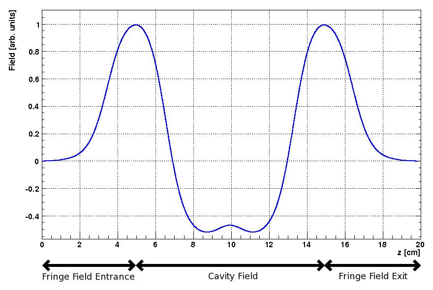
An example of a 1D TRAVELINGWAVE structure field map is shown in
Figure [FINSB-RAC-field]. This map is a standing wave solution generated
by Superfish and shows the field on axis for a single accelerating
cavity with the fringe fields of the structure extending to either side.
OPAL-t reads in this field map and constructs the total field of the
TRAVELINGWAVE structure in three parts: the entrance fringe field, the
structure fields and the exit fringe field.
The fringe fields are treated as standing wave structures and are given by:
\begin{aligned}
    \mathbf{E_{entrance}}(\mathbf{r}, t) &= \mathbf{E_{from-map}}(\mathbf{r}) \cdot \mathrm{VOLT} \cdot \cos \left( 2\pi \cdot \mathrm{FREQ} \cdot t
        + \phi_{entrance} \right) \\
    \mathbf{E_{exit}}(\mathbf{r}, t) &= \mathbf{E_{from-map}}(\mathbf{r}) \cdot \mathrm{VOLT} \cdot \cos \left( 2\pi \cdot \mathrm{FREQ} \cdot t
        + \phi_{exit} \right)
  \end{aligned}
where VOLT and FREQ are the field magnitude and
frequency attributes (see below).
\phi_{entrance}= \mathrm{LAG}, the phase attribute
of the element (see below). \phi_{exit} is dependent
upon both LAG and the NUMCELLS attribute (see below) and is calculated
internally by OPAL-t.
The field of the main accelerating structure is reconstructed from the center section of the standing wave solution shown in Figure [FINSB-RAC-field] using
\begin{aligned}
    \mathbf{E} ( \mathbf{r},t ) &= \frac{\mathrm{VOLT}}{\sin (2 \pi \cdot \mathrm{MODE})} \\
    & \times \Biggl\{ \mathbf{E_{from-map}} (x,y,z) \cdot \cos \biggl( 2 \pi \cdot \mathrm{FREQ} \cdot t + \mathrm{LAG}+ \frac{\pi}{2} \cdot \mathrm{MODE} \Bigr) + \\
    & \mathbf{E_{from-map}}(x,y,z+d) \cdot \cos \biggl( 2 \pi \cdot \mathrm{FREQ} \cdot t + \mathrm{LAG} + \frac{3 \pi}{2} \cdot \mathrm{MODE} \Bigr) \Biggr\}
  \end{aligned}
where d is the cell length and is defined as
\text{d} = \lambda \cdot \mathrm{MODE} . MODE is an
attribute of the element (see below). When calculating the field from
the map (\mathbf{E_{from-map}}(x,y,z)), the longitudinal
position is referenced to the start of the cavity fields at
\frac{\lambda}{2} (In this case starting at
z = {5.0}cm). If the longitudinal position advances past
the end of the cavity map (\frac{3\lambda}{2} = {15.0}cm
in this example), an integer number of cavity wavelengths is subtracted
from the position until it is back within the map’s longitudinal range.
A TRAVELINGWAVE structure has seven real attributes, one integer
attribute, one string attribute and one Boolean attribute:
label:TRAVELINGWAVE, APERTURE=real-vector, L=real,
      VOLT=real, LAG=real, FMAPFN=string,
      ELEMEDGE=real, FREQ=real, NUMCELLS=integer,
      MODE=real;
- L
-
The length of the cavity (default: 0 m). In OPAL-t this attribute is ignored, the length is defined by the field map and the number of cells.
- VOLT
-
The peak RF voltage (default: 0 MV). The effect of the cavity is
\delta E=\mathrm{VOLT}\cdot\sin(\mathrm{LAG}- 2\pi\cdot\mathrm{FREQ}\cdot t). - LAG
-
The phase lag [rad] (default: 0). In OPAL-t this phase is in general relative to the phase at which the reference particle gains the most energy. This phase is determined using an auto-phasing algorithm (see Appendix [autophasing]). This auto-phasing algorithm can be switched off, see
APVETO. - FMAPFN
-
Field maps in the T7 format can be specified.
- FREQ
-
Defines the frequency of the traveling wave structure in units of MHz. A warning is issued when the frequency of the cavity card does not correspond to the frequency defined in the FMAPFN file. The frequency defined in the FMAPFN file overrides the frequency defined on the cavity card.
- NUMCELLS
-
Defines the number of cells in the tank. (The cell count should not include the entry and exit half cell fringe fields.)
- MODE
-
Defines the mode in units of
2\pi, for example\frac{1}{3}stands for a\frac{2 \pi}{3}structure. - FAST
-
If FAST is true and the provided field map is in 1D then a 2D field map is constructed from the 1D on-axis field, see Section [fieldmaps]. To track the particles the field values are interpolated from this map instead of using an FFT based algorithm for each particle and each step. (default: FALSE)
- APVETO
-
If
TRUEthis cavity will not be auto-phased. Instead the phase of the cavity is equal toLAGat the arrival time of the reference particle (arrival at the limit of its field not atELEMEDGE).
Use of a traveling wave requires the particle momentum P and the
particle charge CHARGE to be set on the relevant optics command before
any calculations are performed.
Example of a L-Band traveling wave structure:
lrf0: TravelingWave, L=0.0253, VOLT=14.750,
      NUMCELLS=40, ELEMEDGE=2.73066,
      FMAPFN="INLB-02-RAC.Ez", MODE=1/3,
      FREQ=1498.956, LAG=248.0/360.0;
1.17. Monitor
A MONITOR detects all particles passing it and writes the position,
the momentum and the time when they hit it into an H5hut file.
Furthermore the exact position of the monitor is stored. It has always a
length of 1cm consisting of 0.5cm drift, the monitor of zero length and
another 0.5cm drift. This is to prevent OPAL-t from missing any
particle. The positions of the particles on the monitor are interpolated
from the current position and momentum one step before they would passe
the monitor.
- OUTFN
-
The file name into which the monitor should write the collected data. The file is an H5hut file.
If the attribute TYPE is set to TEMPORAL then the data of all
particles are written to the H5hut file when the reference particle hits
the monitor.
This is a restricted feature: DOPAL-cycl.
1.18. Collimators
Three types of collimators are defined:
- ECOLLIMATOR
-
[sec:ecollimator] Elliptic aperture,
- RCOLLIMATOR
-
[sec:rcollimator] Rectangular aperture.
- CCOLLIMATOR
-
Radial rectangular collimator in cyclotrons
label:ECOLLIMATOR, TYPE=string, APERTURE=real-vector,
      L=real, XSIZE=real, YSIZE=real;
label:RCOLLIMATOR,TYPE=string, APERTURE=real-vector,
      L=real, XSIZE=real, YSIZE=real;
Either type has three real attributes:
- L
-
The collimator length (default: 0 m).
- XSIZE
-
The horizontal half-aperture (default: unlimited).
- YSIZE
-
The vertical half-aperture (default: unlimited).
For elliptic apertures, XSIZE and YSIZE denote the half-axes
respectively, for rectangular apertures they denote the half-width of
the rectangle. Optically a collimator behaves like a drift space, but
during tracking, it also introduces an aperture limit. The aperture is
checked at the entrance. If the length is not zero, the aperture is also
checked at the exit.
Example:
COLLIM:ECOLLIMATOR, L=0.5, XSIZE=0.01, YSIZE=0.005;
The reference system for a collimator is a Cartesian coordinate system
1.18.1. OPAL-t mode
The CCOLLIMATOR isn’t supported. ECOLLIMATORs and RCOLLIMATORs
detect all particles which are outside the aperture defined by XSIZE
and YSIZE. Lost particles are saved in an H5hut file defined by
OUTFN. The ELEMEDGE defines the location of the collimator and L
the length.
- OUTFN
-
The file name into which the monitor should write the collected data. The file is an H5hut file.
Example:
Col:ECOLLIMATOR, L=1.0E-3, ELEMEDGE=3.0E-3, XSIZE=5.0E-4,
    YSIZE=5.0E-4, OUTFN="Coll.h5";
1.18.2. OPAL-cycl mode
Only CCOLLIMATOR is available for OPAL-cycl. This element is radial
rectangular collimator which can be used to collimate the radial tail
particles. So when a particle hit this collimator, it will be absorbed
or scattered, the algorithm is based on the Monte Carlo method . Pleased
note when a particle is scattered, it will not be recorded as the lost
particle. If this particle leave the bunch, it will be removed during
the integration afterwards, so as to maintain the accuracy of space
charge solving.
- XSTART
-
The x coordinate of the start point. [mm]
- XEND
-
The x coordinate of the end point. [mm]
- YSTART
-
The y coordinate of the start point. [mm]
- YEND
-
The y coordinate of the end point. [mm]
- ZSTART
-
The vertical coordinate of the start point [mm]. Default value is -100mm.
- ZEND
-
The vertical coordinate of the end point. [mm]. Default value is -100mm.
- WIDTH
-
The width of the septum. [mm]
- PARTICLEMATTERINTERACTION
-
PARTICLEMATTERINTERACTIONis an attribute of the element. Collimator physics is only a kind of particlematterinteraction. It can be applied to any element. If the type ofPARTICLEMATTERINTERACTIONisCOLLIMATOR, the material is defined here. The material "Cu", "Be", "Graphite" and "Mo" are defined until now. If this is not set, the particle matter interaction module will not be activated. The particle hitting collimator will be recorded and directly deleted from the simulation.

Example:
REAL y1=-0.0;
REAL y2=0.0;
REAL y3=200.0;
REAL y4=205.0;
REAL x1=-215.0;
REAL x2=-220.0;
REAL x3=0.0;
REAL x4=0.0;
cmphys:particlematterinteraction, TYPE="Collimator", MATERIAL="Cu";
cma1: CCollimator, XSTART=x1, XEND=x2,YSTART=y1, YEND=y2,
ZSTART=2, ZEND=100, WIDTH=10.0, PARTICLEMATTERINTERACTION=cmphys ;
cma2: CCollimator, XSTART=x3, XEND=x4,YSTART=y3, YEND=y4,
 ZSTART=2, ZEND=100, WIDTH=10.0, PARTICLEMATTERINTERACTION=cmphys;
The particles lost on the CCOLLIMATOR are recorded in the ASCII file <inputfilename>.loss
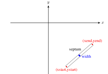
1.19. Septum (OPAL-cycl)
This is a restricted feature: DOPAL-t. The particles hitting on the
septum is removed from the bunch. There are 5 parameters to describe a
septum.
- XSTART
-
The x coordinate of the start point. [mm]
- XEND
-
The x coordinate of the end point. [mm]
- YSTART
-
The y coordinate of the start point. [mm]
- YEND
-
The y coordinate of the end point. [mm]
- WIDTH
-
The width of the septum. [mm]
Example:
eec2: Septum, xstart=4100.0, xend=4300.0,
ystart=-1200.0, yend=-150.0, width=0.05;
The particles lost on the SEPTUM are recorded in the ASCII file <input_file_name >.loss.
1.20. Probe (OPAL-cycl)
The particles hitting on the probe is recorded. There are 5 parameters to describe a probe.
- XSTART
-
The x coordinate of the start point. [mm]
- XEND
-
The x coordinate of the end point. [mm]
- YSTART
-
The y coordinate of the start point. [mm]
- YEND
-
The y coordinate of the end point. [mm]
- WIDTH
-
The width of the probe, NOT used yet.

Example:
prob1: Probe, xstart=4166.16, xend=4250.0,
ystart=-1226.85, yend=-1241.3;
The particles probed on the PROBE are recorded in the ASCII file <inputfilename>.loss. Please note that these particles are not deleted in the simulation, however, they are recorded in the "loss" file.
1.21. Stripper (OPAL-cycl)
A stripper element strip the electron(s) from a particle. The particle hitting the stripper is recorded in the file, which contains the time, coordinates and momentum of the particle at the moment it hit the stripper. The charge and mass are changed. Its has the same geometry as the PROBE element. Please note that the stripping physics in not included yet.
There are 9 parameters to describe a stripper.
- XSTART
-
The x coordinate of the start point. [mm]
- XEND
-
The x coordinate of the end point. [mm]
- YSTART
-
The y coordinate of the start point. [mm]
- YEND
-
The y coordinate of the end point. [mm]
- WIDTH
-
The width of the probe, NOT used yet.
- OPCHARGE
-
Charge number of the out-coming particle. Negative value represents negative charge.
- OPMASS
-
Mass of the out-coming particles. [
\mathrm{GeV/c^2}] - OPYIELD
-
Yield of the out-coming particle (the outcome particle number per income particle) , the default value is 1.
- STOP
-
If STOP is true, the particle is stopped and deleted from the simulation; Otherwise, the out-coming particle continues to be tracked along the extraction path.
Example: H_2^+ particle stripping
prob1: Stripper, xstart=4166.16, xend=4250.0,
ystart=-1226.85, yend=-1241.3,
opcharge=1, opmass=PMASS, opyield=2, stop=false;
No matter what the value of STOP is, the particles hitting on the STRIPPER are recorded in the ASCII file <inputfilename>.loss.
1.22. Degrader (OPAL-t)
Elliptical degrader with an overall length L.
- XSIZE
-
Major axis of the transverse elliptical shape, default value is 1e6.
- YSIZE
-
Minor axis of the transverse elliptical shape, default value is 1e6.
Example: Graphite degrader of 15cm thickness.
DEGPHYS: PARTICLEMATTERINTERACTION, TYPE="DEGRADER", MATERIAL="Graphite";

DEG1: DEGRADER, L=0.15, ELEMEDGE=0.02, PARTICLEMATTERINTERACTION=DEGPHYS;
1.23. Correctors (OPAL-t)
Three types of correctors are available:
- HKICKER
-
[sec:hkicker] A corrector for the horizontal plane.
- VKICKER
-
[sec:vkicker] A corrector for the vertical plane.
- KICKER
-
[sec:kicker] A corrector for both planes.
They act as
label:HKICKER, TYPE=string, APERTURE=real-vector,
      L=real, KICK=real;
label:VKICKER, TYPE=string, APERTURE=real-vector,
      L=real, KICK=real;
label:KICKER, TYPE=string, APERTURE=real-vector,
      L=real, HKICK=real, VKICK=real;
They have the following attributes:
- L
-
The length of the closed orbit corrector (default: 0 m).
- KICK
-
The kick angle in rad for either horizontal or vertical correctors (default: 0rad).
- HKICK
-
The horizontal kick angle in rad for a corrector in both planes (default: 0rad).
- VKICK
-
The vertical kick angle in rad for a corrector in both planes (default: 0rad).
- DESIGNENERGY
-
Fix the magnitude of the magnetic field using the given
DESIGNENERGYand the angle (KICK,HKICKorVKICK). If the designenergy isn’t set then the actual energy of the reference particle at the position of the corrector is used. TheDESIGNENERGYis expected in MeV.
A positive kick increases p_{x} or p_{y}
respectively. Use KICK for an HKICKER or VKICKER and HKICK and
VKICK for a KICKER. Instead of using a KICKER or a VKICKER one
could use an HKICKER and rotate it appropriately using PSI.
Correctors don’t change the reference trajectory. Otherwise they are
implemented as RBEND with \mathrm{E1} = 0 and without
fringe fields (hard edge model). They can be used to model earth’s
magnetic field which is neglected in the design trajectory but which has
a noticeable effect on the trajectory of a bunch at low energies.
Examples:
HK1:HKICKER, KICK=0.001;
VK3:VKICKER, KICK=0.0005;
KHV:KICKER, HKICK=0.001, VKICK=0.0005;
The reference system for an orbit corrector is a Cartesian coordinate system.