1. Physics Models Used in the Particle Matter Interaction Model
The command to define the particle matter interacton is PARTICLEMATTERINTERACTION.
- MATERIAL
-
The material of the surface.
- ENABLERUTHERFORD
-
Switch to disable Rutherford scattering, default true.
The so defined instance has then to be added to an element using the attribute
1.1. The Energy Loss
The energy loss is simulated using the Bethe-Bloch equation.
-\frac{\mathrm{d} E}{\mathrm{d} x}=\frac{K z^2 Z}{A \beta^2}\left[\frac{1}{2} \ln{\frac{2 m_e c^2\beta^2 \gamma^2 Tmax}{I^2}}-\beta^2 \right],where Z is the atomic number of absorber, A
is the atomic mass of absorber, m_e is the electron mass,
z is the charge number of the incident particle,
K=4\pi N_Ar_e^2m_ec^2, r_e is the classical
electron radius, N_A is the Avogadro’s number,
I is the mean excitation energy. \beta and
\gamma are kinematic variables. T_{max} is
the maximum kinetic energy which can be imparted to a free electron in a
single collision.
T_{max}=\frac{2m_ec^2\beta^2\gamma^2}{1+2\gamma m_e/M+(m_e/M)^2},where M is the incident particle mass.
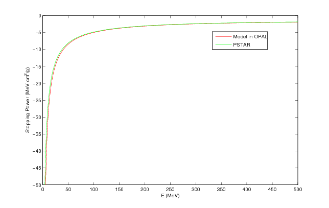
The stopping power is compared with PSTAR program of NIST in Figure 1.
Energy straggling: For relatively thick absorbers such that the number
of collisions is large, the energy loss distribution is shown to be
Gaussian in form. For non-relativistic heavy particles the spread
\sigma_0 of the Gaussian distribution is calculated by:
\sigma_0^2=4\pi N_Ar_e^2(m_ec^2)^2\rho\frac{Z}{A}\Delta s,where \rho is the density, \Delta s is the
thickness.
1.2. The Coulomb Scattering
The Coulomb scattering is treated as two independent events: the
multiple Coulomb scattering and the large angle Rutherford scattering.
Using the distribution given in Classical Electrodynamics, by J. D.
Jackson, the multiple- and single-scattering distributions can be
written:
P_M(\alpha) \;\mathrm{d} \alpha=\frac{1}{\sqrt{\pi}}e^{-\alpha^2}\;\mathrm{d}\alpha,P_S(\alpha) \;\mathrm{d} \alpha=\frac{1}{8 \ln(204 Z^{-1/3})} \frac{1}{\alpha^3}\;\mathrm{d}\alpha,where
\alpha=\frac{\theta}{<\Theta^2>^{1/2}}=\frac{\theta}{\sqrt 2 \theta_0}.
The transition point is
\theta=2.5 \sqrt 2 \theta_0\approx3.5 \theta_0,
\theta_0=\frac{{13.6}{MeV}}{\beta c p} z \sqrt{\Delta s/X_0} [1+0.038 \ln(\Delta s/X_0)],where p is the momentum, \Delta s is the
step size, and X_0 is the radiation length.
1.2.1. Multiple Coulomb Scattering
Generate two independent Gaussian random variables with mean zero and
variance one: z_1 and z_2. If
z_2 \theta_0>3.5 \theta_0, start over. Otherwise,
x=x+\Delta s p_x+z_1 \Delta s \theta_0/\sqrt{12}+z_2 \Delta s \theta_0/2,p_x=p_x+z_2 \theta_0.Generate two independent Gaussian random
variables with mean zero and variance one: z_3 and
z_4. If z_4 \theta_0>3.5 \theta_0, start
over. Otherwise,
y=y+\Delta s p_y+z_3 \Delta s \theta_0/\sqrt{12}+z_4 \Delta s \theta_0/2,p_y=p_y+z_4 \theta_0.1.2.2. Large Angle Rutherford Scattering
Generate a random number \xi_1, if
\xi_1 < \frac{\int_{2.5}^\infty P_S(\alpha)d\alpha}{\int_{0}^{2.5} P_M(\alpha)\;\mathrm{d}\alpha+\int_{2.5}^\infty P_S(\alpha)\;\mathrm{d}\alpha}=0.0047,
sampling the large angle Rutherford scattering.
The cumulative distribution function of the large angle Rutherford scattering is
F(\alpha)=\frac{\int_{2.5}^\alpha P_S(\alpha) \;\mathrm{d} \alpha}{\int_{2.5}^\infty P_S(\alpha) \;\mathrm{d} \alpha}=\xi,where \xi is a random variable. So
\alpha=\pm 2.5 \sqrt{\frac{1}{1-\xi}}=\pm 2.5 \sqrt{\frac{1}{\xi}}.Generate a random variable P_3,
if P_3>0.5
\theta_{Ru}=2.5 \sqrt{\frac{1}{\xi}} \sqrt{2}\theta_0,else
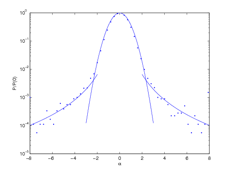
\theta_{Ru}=-2.5 \sqrt{\frac{1}{\xi}} \sqrt{2}\theta_0.The angle distribution after Coulomb scattering is shown in
Figure 2. The line is from Jackson’s formula, and the points are
simulations with Matlab. For a thickness of \Delta s=1e-4
m, \theta=0.5349 \alpha (in degree).
1.3. The Flow Diagram of CollimatorPhysics Class in OPAL
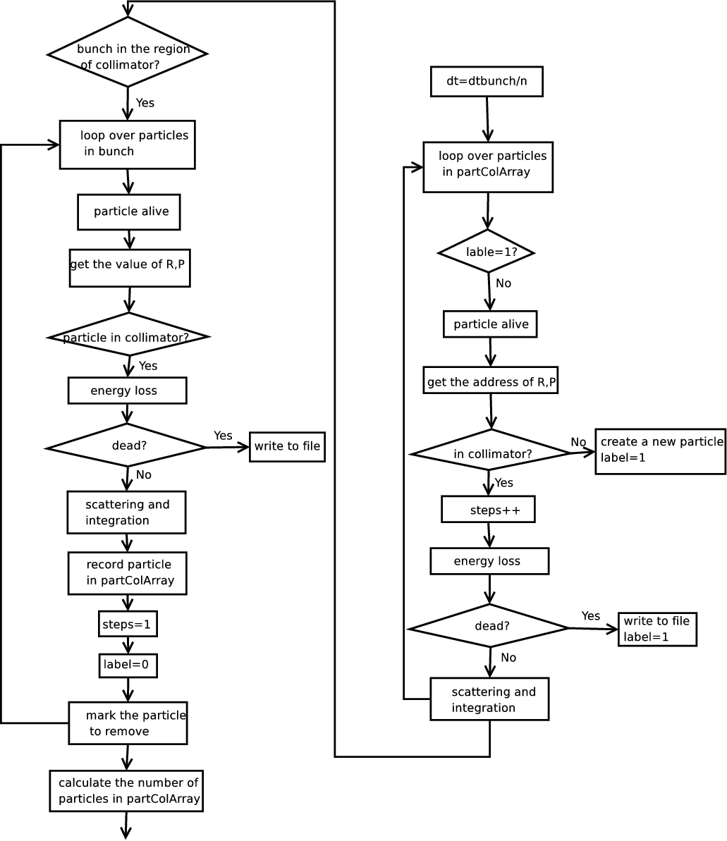
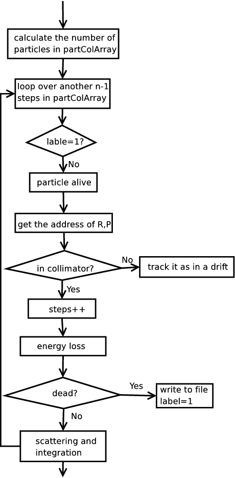
1.3.1. The Substeps
Small step is needed in the routine of CollimatorPhysics.
If a large step is given in the main input file, in the file
CollimatorPhysics.cpp, it is divided by a integer number
n to make the step size using for the calculation of
collimator physics less than 1.01e-12 s. As shown by
Figures 3 and 4 in the previous section, first we track one
step for the particles already in the collimator and the newcomers, then
another (n-1) steps to make sure the particles in the collimator
experience the same time as the ones in the main bunch.
Now, if the particle leave the collimator during the (n-1) steps, we track it as in a drift and put it back to the main bunch when finishing (n-1) steps.
1.4. Available Materials in OPAL
| Material | Z | A |
\rho [g/cm^3] |
X0
[g/cm^2] |
A2 | A3 | A4 | A5 | OPAL Name |
|---|---|---|---|---|---|---|---|---|---|
Aluminum |
13 |
26.98 |
2.7 |
24.01 |
4.739 |
2766 |
164.5 |
2.023E-02 |
|
AluminaAl2O3 |
50 |
101.96 |
3.97 |
27.94 |
7.227 |
11210 |
386.4 |
4.474e-3 |
|
Copper |
29 |
63.54 |
8.96 |
12.86 |
4.194 |
4649 |
81.13 |
2.242E-02 |
|
Graphite |
6 |
12.0172 |
2.210 |
42.7 |
2.601 |
1701 |
1279 |
1.638E-02 |
|
GraphiteR6710 |
6 |
12.0172 |
1.88 |
42.7 |
2.601 |
1701 |
1279 |
1.638E-02 |
|
Titan |
22 |
47.8 |
4.54 |
16.16 |
5.489 |
5260 |
651.1 |
8.930E-03 |
|
Air |
7 |
14 |
0.0012 |
37.99 |
3.350 |
1683 |
1900 |
2.513E-02 |
|
Kapton |
6 |
12 |
1.4 |
39.95 |
2.601 |
1701 |
1279 |
1.638E-02 |
|
Gold |
79 |
197 |
19.3 |
6.46 |
5.458 |
7852 |
975.8 |
2.077E-02 |
|
Water |
10 |
18 |
1 |
36.08 |
2.199 |
2393 |
2699 |
1.568E-02 |
|
Mylar |
6.702 |
12.88 |
1.4 |
39.95 |
3.35 |
1683 |
1900 |
2.513E-02 |
|
Berilium |
4 |
9.012 |
1.848 |
65.19 |
2.590 |
966.0 |
153.8 |
3.475E-02 |
|
Molybdenum |
42 |
95.94 |
10.22 |
9.8 |
7.248 |
9545 |
480.2 |
5.376E-03 |
|
1.5. Example of an Input File
KX1IPHYS: ParticleMatterInteraction, TYPE="Collimator",MATERIAL="Copper";

KX2IPHYS: ParticleMatterInteraction, TYPE="Collimator",MATERIAL="Graphite";

KX0I: ECollimator, L=0.09, ELEMEDGE=0.01, APERTURE={0.003,0.003},OUTFN="KX0I.h5",
      PARTICLEMATTERINTERACTION='KX1IPHYS';

FX5:  Slit, L=0.09, ELEMEDGE=0.01, APERTURE={0.005,0.003},
      PARTICLEMATTERINTERACTION='KX2IPHYS';

FX16: Slit, L=0.09, ELEMEDGE=0.01, APERTURE={-0.005,-0.003},
      PARTICLEMATTERINTERACTION='KX2IPHYS';
FX5 is a slit in x direction, the APERTURE is POSITIVE, the first
value in APERTURE is the left part, the second value is the right
part. FX16 is a slit in y direction, the APERTURE is NEGATIVE, the
first value in APERTURE is the down part, the second value is the up
part.
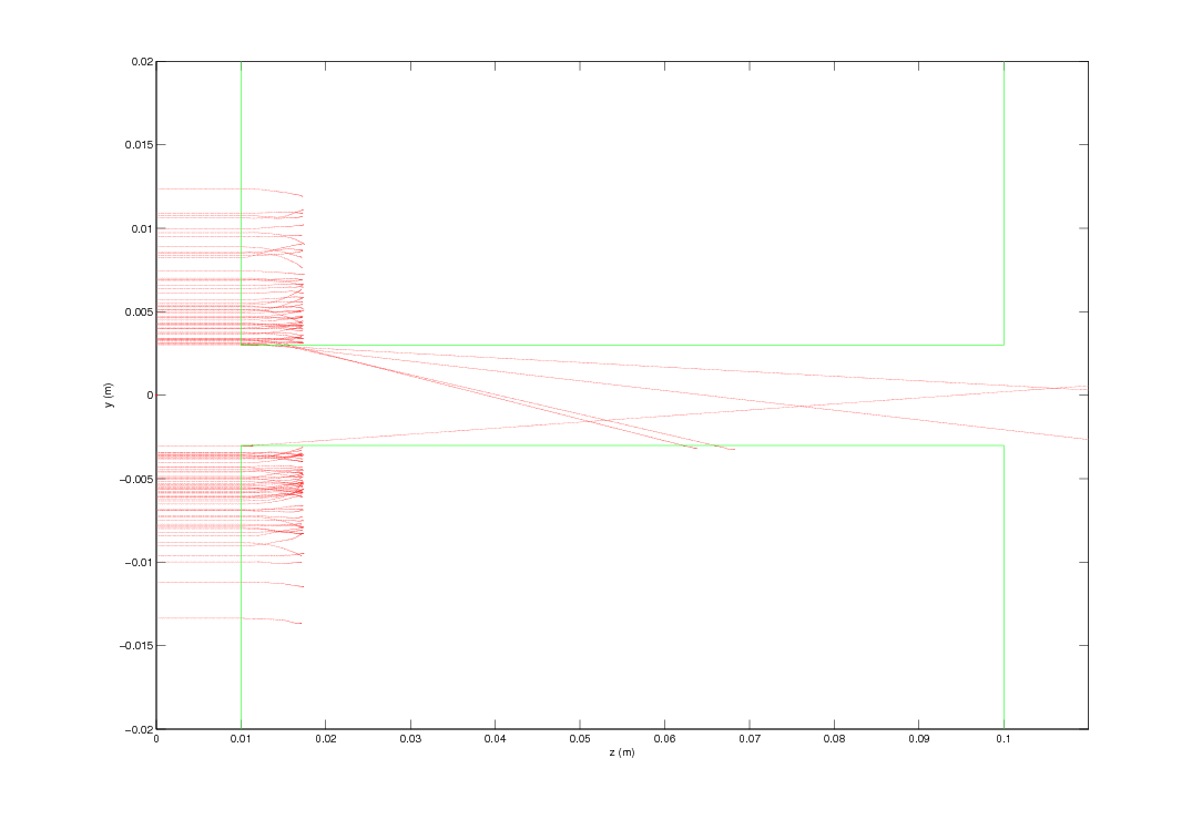
1.6. A Simple Test
A cold Gaussian beam with \sigma_x=\sigma_y=5 mm. The
position of the collimator is from 0.01 m to 0.1 m, the half aperture in
y direction is 3 mm. Figure 5 shows the
trajectory of particles which are either absorbed or deflected by a
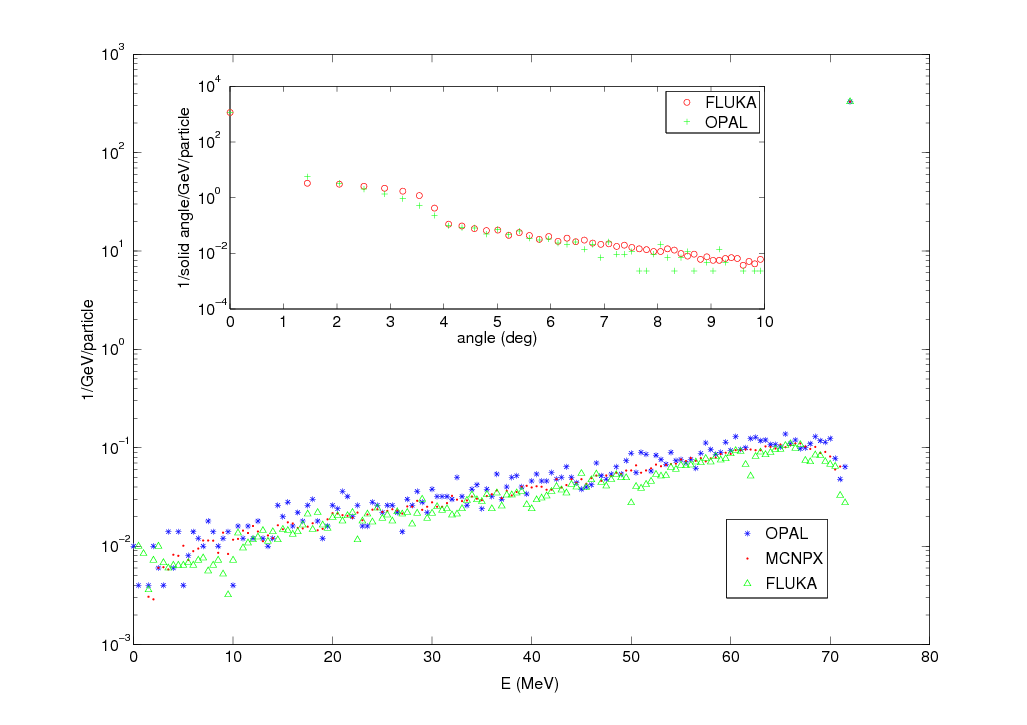
copper slit. As a benchmark of the collimator model in OPAL,
Figure 6 shows the energy spectrum and angle deviation at
z=0.1 m after an elliptic collimator.