tutorial

\$ opal
Ippl> CommMPI: Parent process waiting for children ...
Ippl> CommMPI: Initialization complete.
>                ____  _____       ___
>               / __ \|  __ \ /\   | |
>              | |  | | |__) /  \  | |
>              | |  | |  ___/ /\ \ | |
>              | |__| | |  / ____ \| |____
>               \____/|_| /_/    \_\______|
OPAL >
OPAL > This is OPAL (Object Oriented Parallel Accelerator Library) Version 2.0.0 ...
OPAL >
OPAL > Please send cookies, goodies or other motivations (wine and beer ... )
OPAL > to the OPAL developers opal@lists.psi.ch
OPAL >
OPAL > Time: 16.43.23 date: 30/05/2017
OPAL > Reading startup file "/Users/adelmann/init.opal".
OPAL > Finished reading startup file.
==>

opal input.in --restartfn input.h5 --restart -1 --info 3

-3.5^{\circ}

Option, AUTOPHASE=4;

REAL FINSS_RGUN_phi= (-3.5/180*Pi);

FINSS_RGUN: RFCavity, L = 0.17493, VOLT = 100.0,
    FMAPFN = "FINSS-RGUN.dat",
    ELEMEDGE =0.0, TYPE = "STANDING", FREQ = 2998.0,
    LAG = FINSS_RGUN_phi;

1
FINSS_RGUN
2.22793

Title,string="OBLA Gun";

Option, ECHO=FALSE;
Option, PSDUMPFREQ=10;
Option, VERSION=10600;

REAL Edes=1.0E-9;
REAL gamma=(Edes+EMASS)/EMASS;
REAL beta=sqrt(1-(1/gamma^2));
REAL gambet=gamma*beta;
REAL P0 = gamma*beta*EMASS;
REAL brho = (EMASS*1.0e9*gambet) / CLIGHT;

value,{gamma,brho,Edes,beta,gambet};

// L:        physical element length (real)
// KS:       field scaling factor (real)
// FMAPFN:   field file name (string)
// ELEMEDGE: physical start of the element on the floor (real)
SP1: Solenoid, L=1.20, ELEMEDGE=-0.5335, FMAPFN="1T2.T7",
     KS=0.00011;
SP2: Solenoid, L=1.20, ELEMEDGE=-0.399, FMAPFN="1T3.T7", KS=0.0;
SP3: Solenoid, L=1.20, ELEMEDGE=-0.269, FMAPFN="1T3.T7", KS=0.0;

gun: RFCavity, L=0.011, VOLT=-102.28, FMAPFN="1T1.T7",
     ELEMEDGE=0.00, TYPE="STANDING", FREQ=1.0e-6;

l1:   Line = (gun,sp1,sp2,sp3);

REAL rf=1498.956;
REAL v0=beta*CLIGHT;
REAL lz  = 6.5E-12*v0;
value,{v0,lz};

Dist1:DISTRIBUTION, TYPE=gungauss,
      sigmax=  0.00030, sigmapx=0.0, corrx=0.0,
      sigmay=  0.00030, sigmapy=0.0, corry=0.0,
      sigmat=  lz, sigmapt=1.0, corrt=0.0 ,
      NBIN=39;

Fs1:FIELDSOLVER, FSTYPE=FFT, MX=32, MY=32, MT=32,
                 PARFFTX=true, PARFFTY=true, PARFFTT=false,
                 BCFFTX=open, BCFFTY=open, BCFFTT=open,
                 BBOXINCR=1, GREENSF=STANDARD;

beam1: BEAM, PARTICLE=ELECTRON, pc=P0, NPART=50000,
       BCURRENT=0.008993736, BFREQ=rf, CHARGE=-1;

Select, Line=l1;
track,line=l1, beam=beam1, MAXSTEPS=2000, DT=1.0e-13;
 run, method = "PARALLEL-T", beam=beam1, fieldsolver=Fs1,
      distribution=Dist1;
endtrack;

Stop;

Injector II is a separated sector cyclotron specially designed for pre-acceleration (inject: 870 keV, extract: 72 MeV) of high intensity proton beam for Ring cyclotron. It has 4 sector magnets, two double-gap acceleration cavities (represented by 2 single-gap cavities here) and two single-gap flat-top cavities.

Following is an input file of Single Particle Tracking mode for PSI Injector II cyclotron.

To run opal on a single node, just use this command:

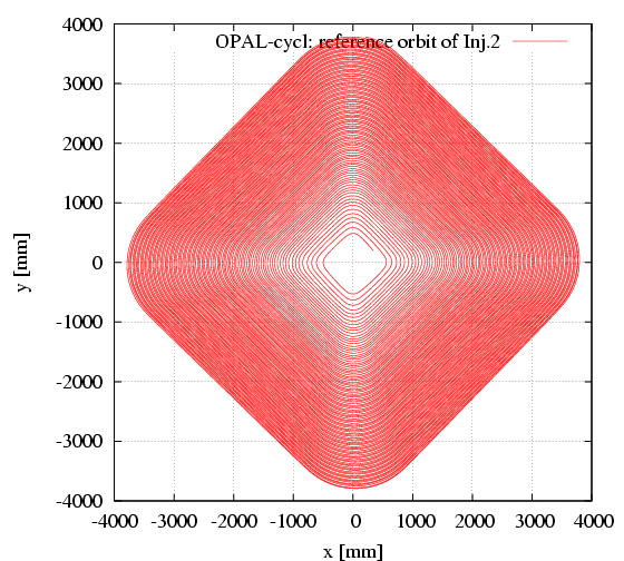
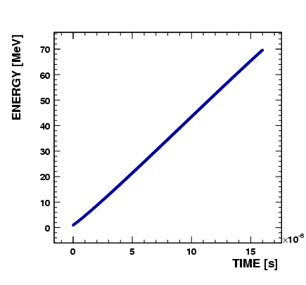
Here shows some pictures using the resulting data from single particle tracking using OPAL-cycl.

Left plot of Figure 1 shows the accelerating orbit of reference particle. After 106 turns, the energy increases from 870 keV at the injection point to 72.16 MeV at the deflection point.

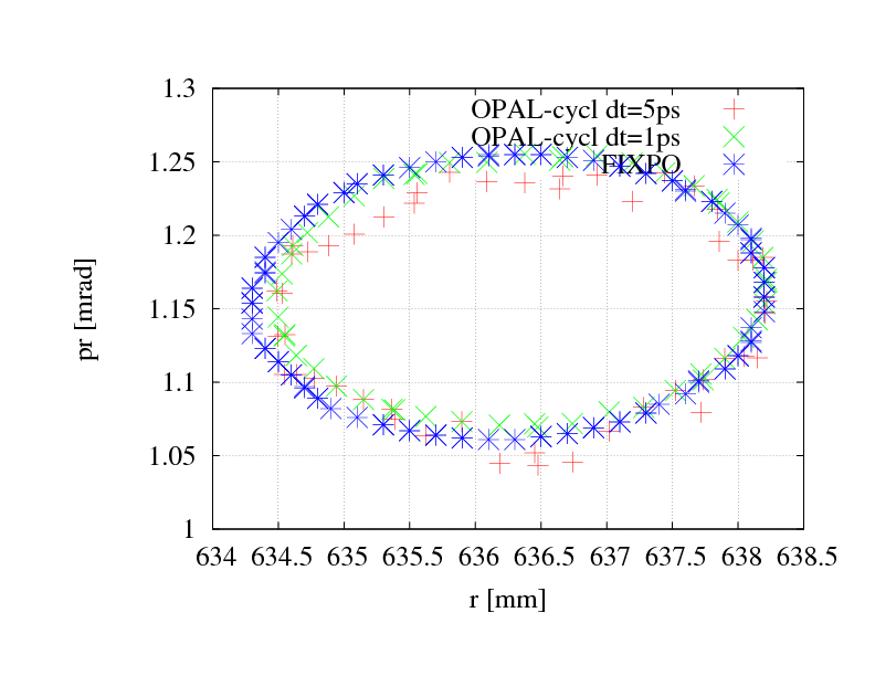
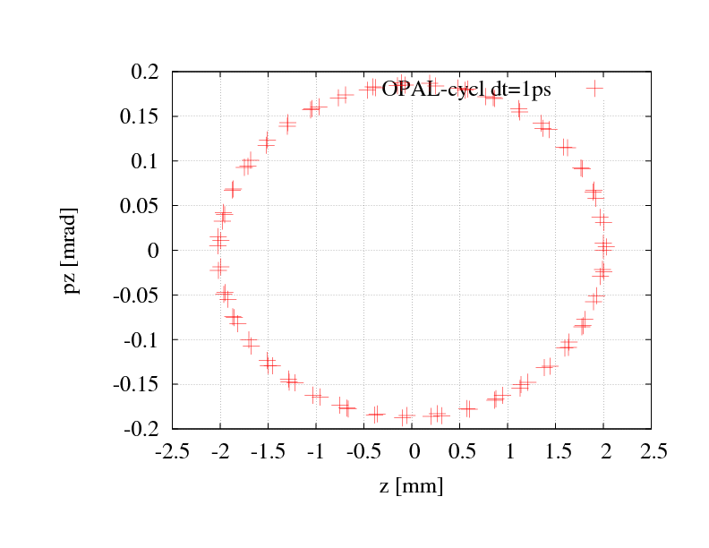
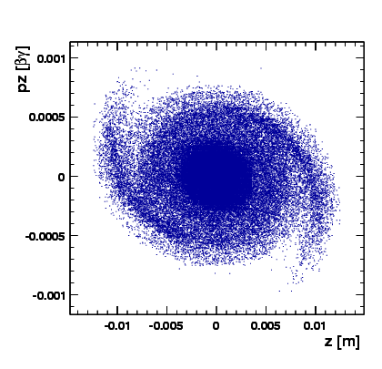
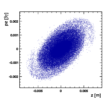
From theoretic view, there should be an eigen ellipse for any given energy in stable area of a fixed accelerator structure. Only when the initial phase space shape matches its eigen ellipse, the oscillation of beam envelop amplitude will get minimal and the transmission efficiency get maximal. We can calculate the eigen ellipse by single particle tracking using betatron oscillation property of off-centered particle as following: track an off-centered particle and record its coordinates and momenta at the same azimuthal position for each revolution. Figure 2 shows the eigen ellipse at symmetric line of sector magnet for energy of 2 MeV in Injector II.

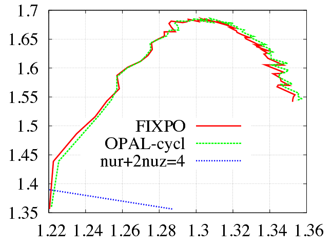
Right plot of Figure 1 shows very good agreement of the tune diagram by OPAL-cycl and FIXPO. The trivial discrepancy should come from the methods they used. In FIXPO, the tune values are obtained according to the crossing points of the initially displaced particle. Meanwhile, in OPAL-cycl, the Fourier analysis method is used to manipulate orbit difference between the reference particle and an initially displaced particle. The frequency point with the biggest amplitude is the betatron tune value at the given energy.

Following is the input file for single bunch tracking with space charge effects in Injector II.

To run opal on single node, just use this command:

To run opal on N nodes in parallel environment interactively, use this command instead:

If restart a job from the last step of an existing .h5 file, add a new argument like this:

Figure 3 and 4 are simulation results, shown by H5ROOT code.

From the view of numerical simulation, the difference between Injector II and Ring cyclotron comes from two aspects:

B Field

The structure of Ring is totally symmetric, the field on median plain is periodic along azimuthal direction, OPAL-cycl take this advantage to only store field data to save memory.

RF Cavity

In the Ring, all the cavities are typically single gap with some parallel displacement from its radial position.OPAL-cycl have an argument PDIS to manipulate this issue.

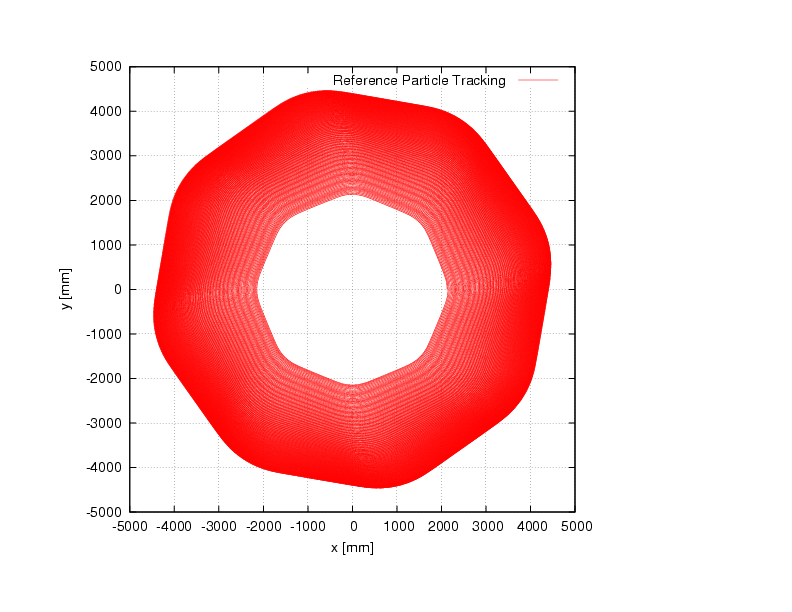
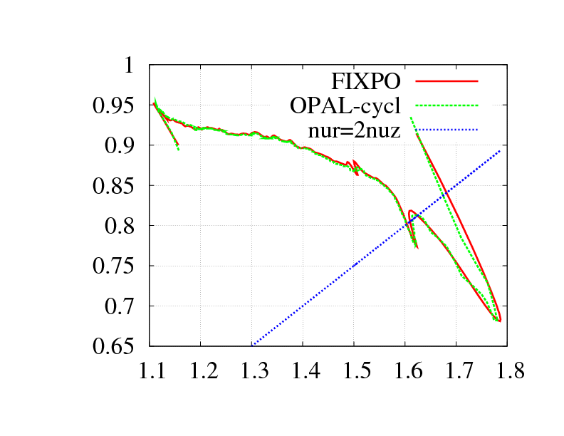
Figure 5 shows a single particle tracking result and tune calculation result in the PSI Ring cyclotron. Limited by size of the user guide, we don’t plan to show too much details as in Injector II.

The GUNGAUSSFLATTOPTH and ASTRAFLATTOPTH distribution types see Section astraflattopthdisttype are two common types previously implemented to simulate electron beams emitted from photocathodes in an electron photoinjector. These are no longer explicitly supported and are instead now defined as specialized sub-types of the distribution type FLATTOP. That is, the emitted distributions represented by GUNGAUSSFLATTOPTH and ASTRAFLATTOPTH can now be easily reproduced by using the FLATTOP distribution type and we would encourage use of the new command structure.

Having said this, however, old input files that use the GUNGAUSSFLATTOPTH and ASTRAFLATTOPTH distribution types will still work as before, with the following exception. Previously, OPAL had a Boolean OPTION command FINEEMISSION (default value was TRUE). This OPTION is no longer supported. Instead you will need to set the distribution attribute EMISSIONSTEPS see Table [distattremitted] to a value that is 10

the value of the distribution attribute NBIN see Table [distattruniversal] in order for your simulation to behave the same as before.

The FROMFILE see Section [fromfiledisttype], GAUSS see Section [gaussdisttype] and BINOMIAL see Section [binomialdisttype] distribution types have changed from previous versions of OPAL. However, legacy distribution commands should work as before with one exception. If you are using OPAL-cycl then your old input files will work just fine. However, if you are using OPAL-t then you will need to set the distribution attribute INPUTMOUNITS see Section [unitsdistattributes] to: