1. Multi Objective Optimisation
Optimization methods deal with finding a feasible set of solutions corresponding to extreme values of some specific criteria. Problems consisting of more than one criterion are called multi-objective optimization problems. Multiple objectives arise naturally in many real world optimization problems, such as portfolio optimization, design, planning and many more [pgnl:06,zepv:00,gala:98,yrss:09,basi:05]. It is important to stress that multi-objective problems are in general harder and more expensive to solve than single-objective optimization problems.
In this chapter we introduce multi-objective optimization problems and discuss techniques for their solution with an emphasis on evolutionary algorithms.
1.1. Definition
As with single-objective optimization problems, multi-object optimization problems consist of a solution vector and optionally a number of equality and inequality constraints. Formally, a general multi-objective optimization problem has the form
\begin{aligned}
  \mathrm{min}  \quad & \quad f_m(\mathbf{x}),        & m &= \{1, \ldots, M\} \\
  \mathrm{s.t.} \quad & \quad g_j(\mathbf{x}) \geq 0, & j &= \{1, \ldots, J\} \\
  \quad & \quad  -\infty \leq x_i^L \leq \mathbf{x}=x_i \leq x_i^U \leq \infty,& i &= \{0, \ldots, n \}.
\end{aligned}
The M
objectives ([eq:moop:obj]) are minimized, subject to J
inequality constraints ([eq:moop:constr]). An n-vector
([eq:moop:dvar]) contains all the design variables with appropriate
lower and upper bounds, constraining the design space.
In contrast to single-objective optimization the objective functions
span a multi-dimensional space in addition to the design variable space
– for each point in design space there exists a point in objective
space. The mapping from the n dimensional design space to
the M dimensional objective space visualized in
Figure [fig:des_to_obj] is often non-linear. This impedes the search for
optimal solutions and increases the computational cost as a result of
expensive objective function evaluation. Additionally, depending in
which of the two spaces the algorithm uses to determine the next step,
it can be difficult to assure an even sampling of both spaces
simultaneously.
f : \mathbb{R}^n \rightarrow \mathbb{R}^M from design to objective space. The dashed lines represent the constraints in design space and the set of solutions (Pareto front) in objective space.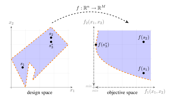
A special subset of multi-objective optimization problems where all objectives and constraints are linear, called Multi-objective linear programs, exhibit formidable theoretical properties that facilitate convergence proofs. In this thesis we strive to address arbitrary multi-objective optimization problems with non-linear constraints and objectives. No general convergence proofs are readily available for these cases.
1.2. Pareto Optimality
In most multi-objective optimization problems we have to deal with conflicting objectives. Two objectives are conflicting if they possess different minima. If all the mimima of all objectives coincide the multi-objective optimization problem has only one solution. To facilitate comparing solutions we define a partial ordering relation on candidate solutions based on the concept of dominance. A solution is said to dominate another solution if it is no worse than the other solution in all objectives and if it is strictly better in at least one objective. A more formal description of the dominance relation is given in Definition [def:dom] [deb:09].
The properties of the dominance relation include transitivity
x_1 \preceq x_2 \wedge x_2 \preceq x_3 \Rightarrow x_1 \preceq x_3 ,and asymmetricity, which is necessary for an unambiguous order relation
x_1 \preceq x_2 \Rightarrow x_2 \npreceq x_1 .Using the concept of dominance, the sought-after set of Pareto optimal solution points can be approximated iteratively as the set of non-dominated solutions.
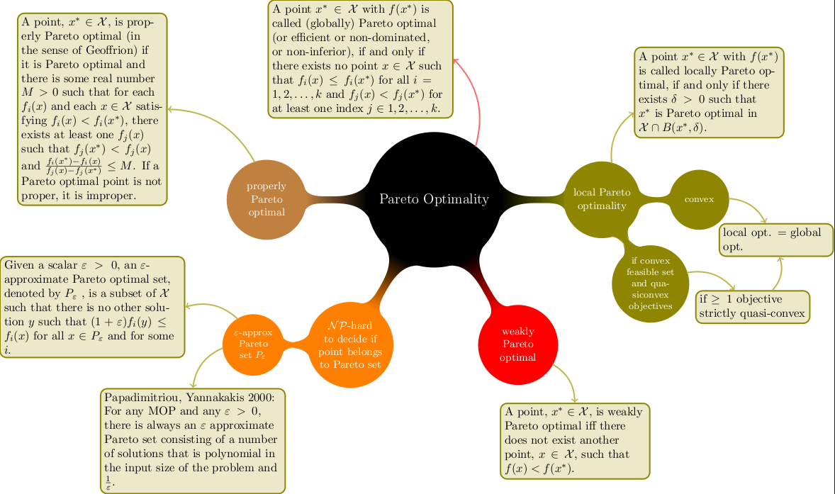
The problem of deciding if a point truly belongs to the Pareto set is
NP-hard. As shown in Figure [fig:pareto-def] there exist "weaker"
formulations of Pareto optimality. Of special interest is the result
shown in [paya:01], where the authors present a polynomial (in the input
size of the problem and 1/\varepsilon) algorithm for
finding an approximation, with accuracy \varepsilon, of
the Pareto set for database queries.