1. Benchmarks
1.1. OPAL-t compared with TRANSPORT & TRACE 3D
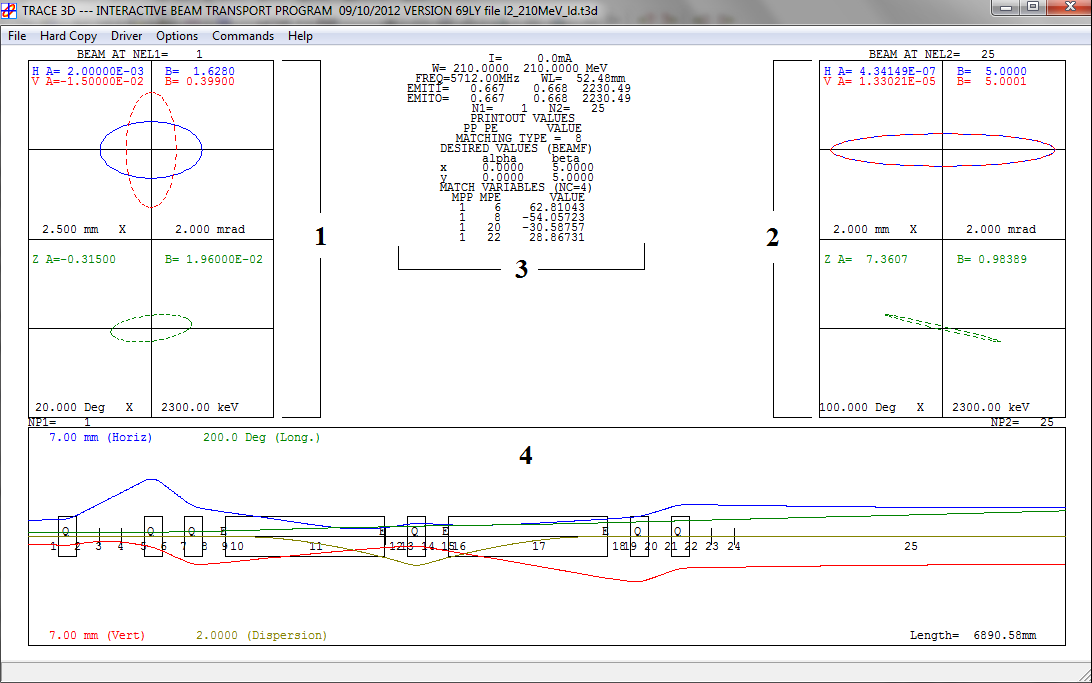
1.1.1. TRACE 3D
TRACE 3D is an interactive beam dynamics program that calculates the envelopes of a bunched beam, including linear space-change forces [Trace_man]. It provides an instantaneous beam profile diagram and delineates the transverse and longitudinal phase plane, where the ellipses are characterized by the Twiss parameters and emittances (total and unnormalized).
1.1.2. TRACE 3D Units
TRACE 3D supports the following internal coordinates and units for the three phase planes:
-
horizontal plane:
x [mm] is the displacement from the center of the beam bunch;
x’ [mrad] is the beam divergence; -
vertical plane:
y [mm] is the displacement from the center of the beam bunch;
y’ [mrad] is the beam divergence; -
longitudinal plane:
z [mm] is the displacement from the center of the beam bunch;
\Deltap/p [mrad] is the difference between the particle’s longitudinal momentum and the reference momentum of the beam bunch.
For input and output, however, z and \Deltap/p are
replaced by \Delta\phi [degree] and \DeltaW
[keV], respectively the displacement in phase and energy. The
relationships between these longitudinal coordinates are:
z = -\frac{\beta\lambda}{360}\Delta\phiand
\frac{\Delta p}{p} = \frac{\gamma}{\gamma +1}\frac{\Delta W}{W}where \beta and \gamma are the relativist
parameters, \lambda is the free-space wavelength of the RF
and W is the kinetic energy [MeV] at the beam center. This internal
conversion can be displayed using the command W (see [Trace_man] page
42).
1.1.3. TRACE 3D Input beam
In TRACE 3D, the input beam is described by the following set of parameters:
-
ER: particle rest mass [MeV/c^{2}];
-
Q: charge state (+1 for protons);
-
W: beam kinetic energy [MeV]
-
XI: beam current [mA]
-
BEAMI: array with initial Twiss parameters in the three phase planes
BEAMI =
\alpha_x , \beta_x, \alpha_y, \beta_y, \alpha_{\phi}, \beta_{\phi}The alphas are dimensionless,
\beta_xand\beta_yare expressed in m/rad (or mm/mrad) and\beta_{\phi}in deg/keV; -
EMITI: initial total and unnormalized emittances in x-x’, y-y’, and
\Delta\phi-\Delta Wplanes.EMITI =
\epsilon_x , \epsilon_y, \epsilon_{\phi}The transversal emittances are expressed in
\pi-mm-mrad and in\pi-deg-keV the longitudinal emittance.
In this beam dynamics code, the total emittance in each phase plane is
five times the RMS emittance in that plane and the displayed beam
envelopes are \sqrt{5}-times their respective RMS values.
TRACE 3D Graphic Interface
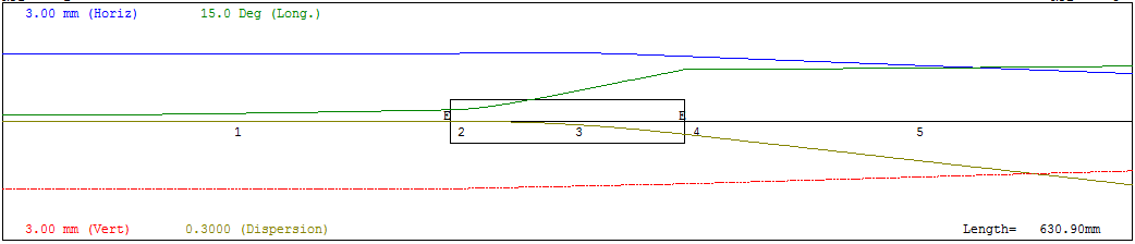
An example of TRACE 3D graphic interface is shown in Figure [trace].
1.1.4. TRANSPORT
TRANSPORT is a computer program for first-order and second-order matrix multiplication, intended for the design of beam transport system [bib:transport]. The TRANSPORT version for Windows provides a graphic beam profile diagram, as well as a sigma matrix description of the simulated beam and line [Transport_GUI]. Differently from TRACE 3D, the ellipses are characterized by the sigma-matrix coefficients and the Twiss parameters and emittances (total and unnormalized) are reported as output information.
1.1.5. TRANSPORT Units
At any specified position in the system, an arbitrary charged particle is represented by a vector, whose components are positions, angles and momentum of the particle with respect to the reference trajectory. The standard units and internal coordinates in TRANSPORT are:
-
horizontal plane:
x [cm] is the displacement of the arbitrary ray with respect to the assumed central trajectory;
\theta[mrad] is the angle the ray makes with respect to the assumed central trajectory; -
vertical plane:
y [cm] is the displacement of the arbitrary ray with respect to the assumed central trajectory;
\phi[mrad] is the angle the ray makes with respect to the assumed central trajectory; -
longitudinal plane:
l [cm] is the path length difference between the arbitrary ray and the central trajectory;
\delta[%] is the fractional momentum deviation of the ray from the assumed central trajectory.
Even if TRANSPORT supports this standard set of units [cm, mrad and %]; however using card 15, the users can redefine the units (see page 99 on TRANSPORT documentation [bib:transport] for more details).
1.1.6. TRANSPORT Input beam
The input beam is described in card 1 in terms of the semi-axes of a six-dimensional erect ellipsoid beam. In terms of diagonal sigma-matrix elements, the input beam in TRANSPORT is expressed by 7 parameters:
-
\sqrt{\sigma_{ii}}[cm] represents one-half of the horizontal (i=1), vertical (i=3) and longitudinal extent (i=5); -
\sqrt{\sigma_{ii}}[mrad] represents one-half of the horizontal (i=2), vertical (i=4) beam divergence; -
\sqrt{\sigma_{66}}[%] represents one-half of the momentum spread; -
p(0) is the momentum of the central trajectory [GeV/c].
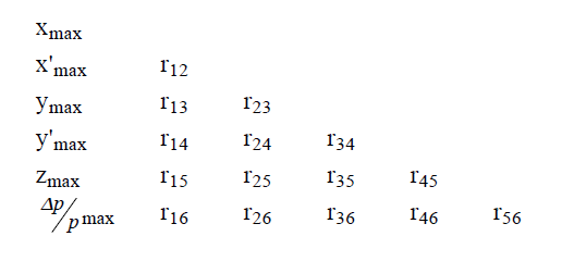
If the input beam is tilted (Twiss alphas not zero), card 12 must be
used, inserting the 15 correlations r_{ij} parameters
among the 6 beam components. The correlation parameters are defined as
following:
r_{ij}=\frac{\sigma_{ij}}{\sqrt{\sigma_{ii}gma_{jj}}}As explained before, with the card 15, it is possible to transform the TRANSPORT standard units in TRACE-like units. In this way, the TRACE 3D sigma-matrix for the input beam, printed out by command Z, can be directly used as input beam in TRANSPORT. An example of TRACE 3D sigma-matrix structure is shown in Figure [trace_z].
From the sigma-matrix coefficients, TRANSPORT reports in output the Twiss parameters and the total, unnormalized emittance. Even in this case, a factor 5 is present between the emittances calculated by TRANSPORT and the corresponding RMS values.
TRANSPORT Graphic Interface
An improved version of TRANSPORT has been embedded in a new graphic shell written in C++ and is providing GUI type tools, which makes it easier to design new beam lines. A screen shot of a modern GUI Transport interface [Transport_GUI] is shown in Figure [TRANSPORT].
1.1.7. Comparison TRACE 3D and TRANSPORT
This study has been done following the same trend of the Regression Test in OPAL [AMAS], replacing the electron beam with a same energy proton beam. Due to the different beam rigidity, the bending magnet features have been redefined with a new magnetic field.
The simulated beam transport line contains:
-
drift space (DRIFT 1): 0.250 m length;
-
bending magnet (SBEND or RBEND): 0.250 m radius of curvature;
-
drift space (DRIFT 2): 0.250 m length.
Keeping fixed the lattice structure, many similar transport lines have been tested adding entrance and exit edge angles to the bending magnet, changing the bending plane (vertical bending magnet) and direction (right or left). In all the cases, the difficulties arise from the non-achromaticity of the system and an increase in the horizontal and longitudinal emittance is expected. In addition, the coupling between these two planes has to be accurately studied.
In the following paragraph, an example of Sector Bending magnet (SBEND) simulation with entrance and exit edge angles is discussed.
Input beam
The starting simulation has been performed with TRACE 3D code. According to Section [T3D_input], the simulated input beam is described by the following parameters:
ER = 938.27
W = 7
FREQ = 700
BEAMI = 0.0, 4.0,0.0, 4.0, 0.0, 0.0756
EMITI = 0.730, 0.730, 7.56
Thanks to the TRACE 3D graphic interface, the input beam can immediately be visualized in the three phase plane as shown in Figure [Input_TRACE].

The corresponding sigma-matrix with the relative units is displayed by command Z:

Before entering the TRACE 3D sigma-matrix coefficients in TRANSPORT, a changing in the units is required using the card 15 in the following way:
15. 1. 'MM' 0.1 ; //express in mm the horizontal and vertical beam size
15. 5. 'MM' 0.1 ; //express in mm the beam length
At this point, the TRANSPORT input beam is defined by card 1:
1.0 1.709 0.427 1.709 0.427 0.11 0.0717 0.1148 /BEAM/ ;
using exactly the same sigma-matrix coefficients of Figure [TRACE_z_Input]. Other two cards must be added in order to use exactly the TRACE 3D R-matrix formalism:
16. 3. 1863.153; //proton mass, as ratio of electron mass
22. 0.05 0.0 700 0.0 /SPAC/ ; //space charge card
SBEND in TRACE 3D
The bending magnet definition in TRACE 3D requires:
| Parameter | Value | Description |
|---|---|---|
NT |
8 |
Type code for bending |
|
30 |
angle of bend in horizontal plane |
|
250 |
radius of curvature of central trajectory |
n |
0 |
field-index gradient |
vf |
0 |
flag for vertical bending |
The edge angles are described with another type code and parameters which include also the fringe field. They must be added before and after the bending magnet if entrance and exit edge angles are present and if the fringe field has to be taken into account. In particular for the entrance edge angle:
| Parameter | Value | Description |
|---|---|---|
NT |
9 |
Type code for edge |
|
10 |
pole-face rotation |
|
250 |
radius of curvature of central trajectory |
g [mm] |
20 |
total gap of magnet |
|
0.36945 |
fringe-field factor |
|
0.36945 |
fringe-field factor |
A same configuration has been used for exit edge angle using
\beta = {5}{^{\circ}}. The beam envelopes in the three
phase planes for this simulation are shown in Figure [Trace_env].
SBEND in TRANSPORT
The bending magnet definition in TRANSPORT requires:
| Parameter | Value | Description |
|---|---|---|
Card |
4 |
Type code for bending |
L [m] |
30 |
Effective length of the central trajectory |
|
250 |
Central field strength |
n |
0 |
field-index gradient |
As for TRACE 3D, the edge angles are described with another card and parameters. In TRANSPORT, however, the fringe field is not automatically included with the edge angle, but it is described by a own card as reported in the Table [Edge_Trans].
| Parameter | Value | Description |
|---|---|---|
Card |
2 |
Type code for edge |
|
10 |
pole-face rotation |
Card |
16 |
Type code for fringe field |
g [mm] |
10 |
half-gap of magnet |
|
0.36945 |
fringe-field factor |
|
0.36945 |
fringe-field factor |
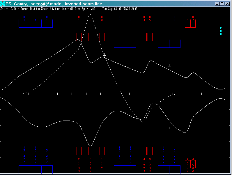
Running the Graphic TRANSPORT version, the beam envelopes in the transverse phase planes for this simulation are shown in Figure [Tran_env].

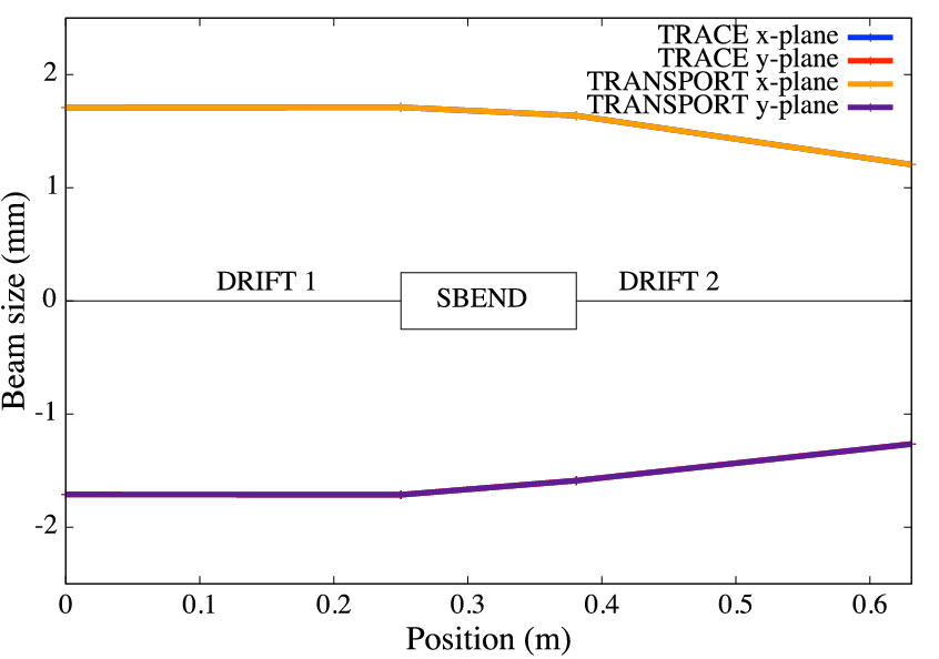
Beam size and emittance comparison
In the next table, the results of the comparison between TRACE 3D and TRANSPORT in terms of the transversal beam sizes at the end of each element in the line are summarized.
Position |
z (m) |
|
|
|
|
Input |
0.000 |
1.709 |
1.709 |
1.709 |
1.709 |
Drift 1 |
0.250 |
1.712 |
1.712 |
1.712 |
1.712 |
Edge |
0.250 |
1.712 |
1.712 |
1.712 |
1.712 |
Bend |
0.381 |
1.638 |
1.587 |
1.638 |
1.587 |
Edge |
0.381 |
1.638 |
1.587 |
1.638 |
1.587 |
Drift 2 |
0.631 |
1.206 |
1.264 |
1.206 |
1.264 |
The perfect agreement between these two codes arises immediately looking at Figure [T3D_Tra_env].
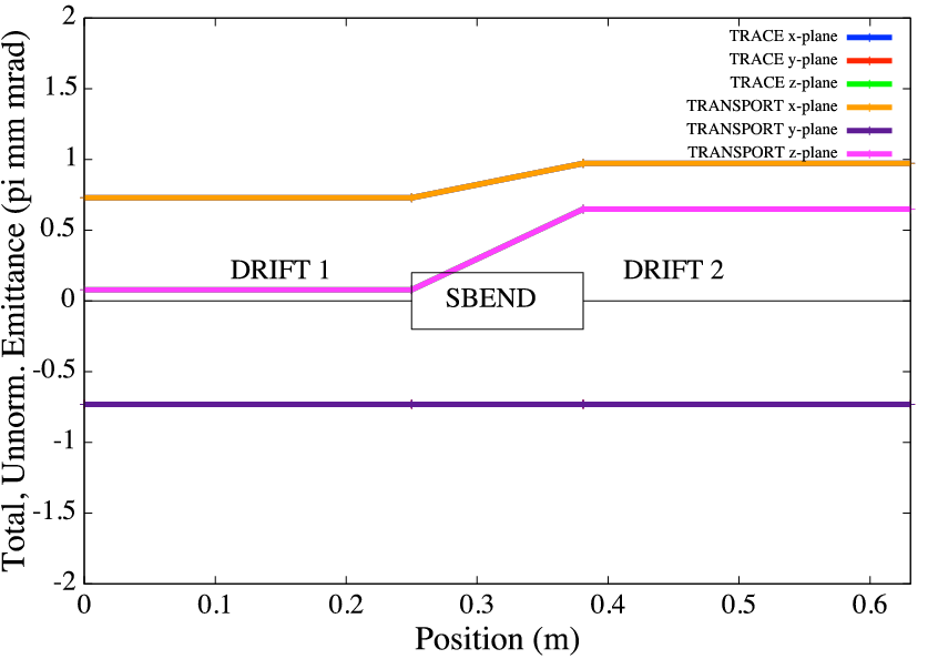
The same comparison has been performed in terms of horizontal and
longitudinal emittance, both expressed in \pi-mm-mrad.
While the vertical emittance remains constant and equal to the initial
value (\epsilon_y = 0.730 \pi-mm-mrad) ,
the horizontal and longitudinal emittances are expected growing after
the bending magnet. The results are reported in Table [Emittance] and in
Figure [T3D_Tra_emi].
Position |
z (m) |
|
|
|
|
Input |
0 |
0.730 |
0.08 |
0.730 |
0.08 |
Drift 1 |
0.250 |
0.730 |
0.08 |
0.730 |
0.08 |
Edge |
0.250 |
0.730 |
0.08 |
0.730 |
0.08 |
Bend |
0.381 |
0.973 |
0.65 |
0.973 |
0.65 |
Edge |
0.381 |
0.973 |
0.65 |
0.973 |
0.65 |
Drift 2 |
0.631 |
0.973 |
0.65 |
0.973 |
0.65 |
From TRACE 3D to TRANSPORT
| Parameter | Trace 3D | Transport |
|---|---|---|
Bend card |
8 |
4 |
Angle |
Input parameter [deg] |
Output information [deg] |
Magn. field |
Calculated. [T] |
Input parameter [kG] |
Radius of curv. |
Input parameter [mm] |
Output information [m] |
Field-index |
Input parameter |
Input parameter |
Effect. length |
Calculated [mm] |
Input parameter [m] |
Edge card |
9 |
2 |
Edge angle |
Input parameter [deg] |
Input parameter [deg] |
Vertical gap |
9 |
16.5 |
Gap |
Total [mm] |
Half-gap [cm] |
Fringe field card |
9 |
16.7 / 16.8 |
|
Default: 0.45 |
Default: 0.5 |
|
Default: 2.8 |
Default: 0 |
Bend direction |
Bend angle sign |
Coord. rotation |
Horiz. right |
Angle |
Angle |
Horiz. left |
Angle |
Card 20 |
Vertical bend |
Card 8, vf |
Card 20 |
1.1.8. Relations to OPAL-t
In OPAL, the beam dynamics approach (time integration) is hence completely different from the envelope-like supported by TRACE 3D and TRANSPORT. The three codes support different units and require diverse parameters for the input beam. A summary of their main features is reported in Table [Features].
| Code | TRACE 3D | TRANSPORT | OPAL |
|---|---|---|---|
Type |
Envelope |
Envelope |
Time integration |
Input |
Twiss, Emittance |
Sigma, Momentum |
Sigma, Energy |
Units |
mm-mrad, deg-keV |
cm-rad, cm-% |
m- |
1.1.9. OPAL-t Units
OPAL-t supports the following internal coordinates and units for the three phase planes:
-
horizontal plane:
X [m] horizontal position of a particle relative to the axis of the element;
PX [\beta_x\gamma] horizontal canonical momentum; -
vertical plane:
Y [m] vertical position of a particle relative to the axis of the element;
PY [\beta_y\gamma] horizontal canonical momentum; -
longitudinal plane:
Z [m] longitudinal position of a particle in floor-coordinates;
PZ [\beta_z\gamma] longitudinal canonical momentum;
1.1.10. OPAL-t Input beam
For the input beam, a GAUSS distribution type has been chosen. For
transferring the TRANSPORT (or TRACE 3D) input beam in terms of
sigma-matrix coefficients, it necessary to:
-
adjust the units: from mm to m;
-
correct for the factor
\sqrt{5}: from total to RMS distribution; -
multiply for the relativistic factor
\beta\gamma ={0.1224}for 7 MeV protons;
In case of the modified sigma-matrix in Figure [TRACE_z_Input], the
corresponding OPAL parameters for the GAUSS distributions are:
 T3D SIGMA                        OPAL -T
-------------------------------------------------------
1.7088 mm             SIGMAX  = 1.7088/sqrt(5)e-3         m
0.4272 mrad           SIGMAPX = 0.4272/sqrt(5)*0.1224e-3
1.7088 mm             SIGMAY  = 1.7088/sqrt(5)e-3        m
0.4272 mrad           SIGMAPY = 0.4272/sqrt(5)*0.1224e-3
0.1092 mm             SIGMAZ  = 0.1092/sqrt(5)e-3        m
0.0717 %              SIGMAPZ = (0.0717*10)/sqrt(5)*0.1224e-3
At the end of this calculation, the input beam in OPAL is:
D1: DISTRIBUTION, TYPE=GAUSS,
SIGMAX = 0.7642e-03,  SIGMAPX= 0.0234e-03,  CORRX= 0.0,
SIGMAY = 0.7642e-03,  SIGMAPY= 0.0234e-03,  CORRY= 0.0,
SIGMAZ = 0.0488e-03,  SIGMAPZ= 0.0392e-03,  CORRZ= 0.0, R61= 0.0,
INPUTMOUNITS=NONE;
1.1.11. Comparison TRACE 3D and OPAL-t
In this section, the comparison between TRACE 3D and OPAL-t is
discussed starting from SBEND definition in OPAL-t. The transport
line described in Section [T3D_TRAN] has been simulated in OPAL using
10.000 particles and 10^{-11} s time step. The bending
magnet features of Table [Bend_Trace,Edge_Trace] have been transformed
in OPAL language as:
Bend: SBEND, ANGLE = 30.0 * Pi/180.0,
             K1=0.0,
             E1=0, E2=0,
             FMAPFN = "1DPROFILE1-DEFAULT",
             ELEMEDGE = 0.250,  // end of first drift
             DESIGNENERGY = 7E+06,  // ref energy eV
             L = 0.1294,
             GAP = 0.02;
-
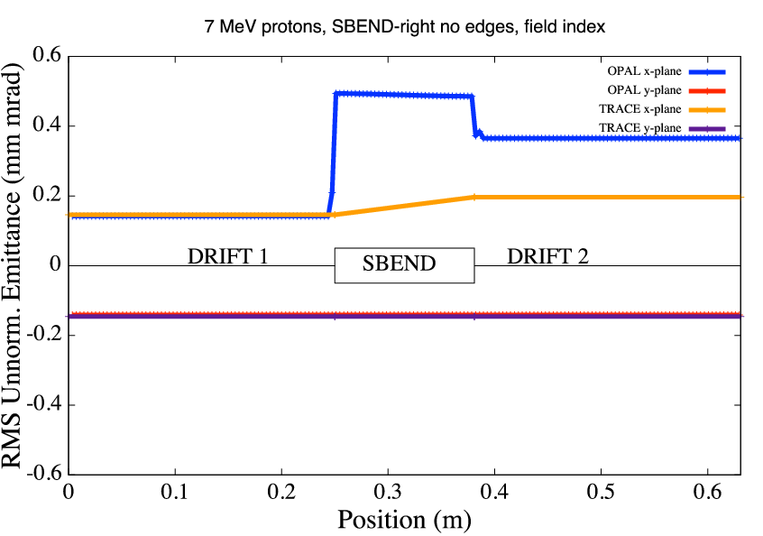
SBEND without edge angles:
// Bending magnet configuration:
K1=0.0,
E1=0, E2=0,
TRACE 3D and OPAL comparison: SBEND without edge angles,
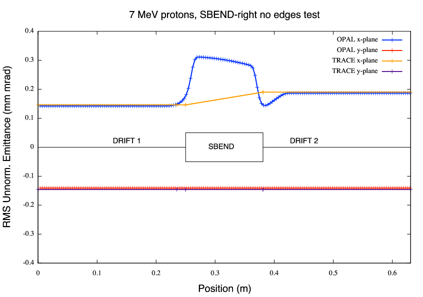
A good overall agreement has been found between the two codes in term of beam size and emittance. The different behavior inside the bending magnet for the horizontal emittance is still undergoing study and it’s probably due to a diverse coordinate system in the two codes.
-
SBEND with edge angles:
// Bending magnet configuration:
K1=0.0,
E1=10*Pi/180.0, E2=5* Pi/180.0,
TRACE 3D and OPAL comparison: SBEND with edge angles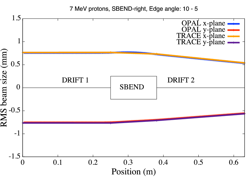

Even in this case, a good overall agreement has been found between the two codes in term of beam size and emittance.
-
SBEND with field index:
The field index parameter K1 is defined as:
K1 = \frac{1}{B\rho}\frac{\partial B_y}{\partial x},Section [RBend]. Instead, in TRACE 3D the field index parameter n is:
n = -\frac{\rho}{B_y}\frac{\partial B_y}{\partial x}.In order to have a significant focusing effect on both transverse planes, the transport line has been simulated in TRACE 3D using
n = 1.5. Since, a different definition exists between OPAL and TRACE 3D on the field index, the n-parameter translation in OPAL language has been done with the following tests:-
TEST 1: K1
=n/\rho^2 -
TEST 2: K1
=n -
TEST 3: K1
=n/\rhoOnly the TEST 2 reports a reasonable behavior on the beam size and emittance, as shown in Figure [SBEND_FI] using:
// Bending magnet configuration:
K1=1.5
E1=0, E2=0,
TRACE 3D and OPAL comparison: SBEND with field index and default field map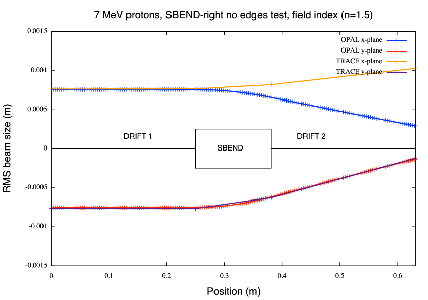
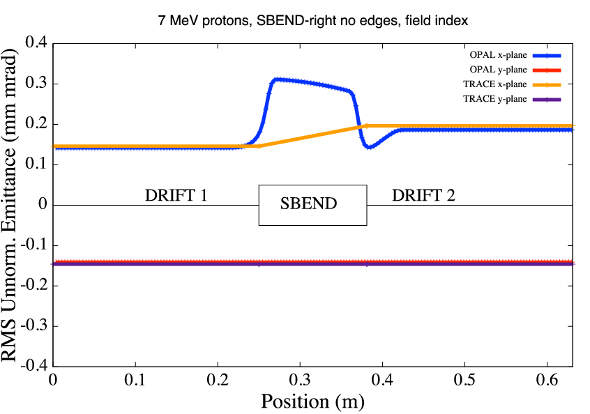
Concerning the emittances and vertical beam size, a perfect agreement has been found, instead a defocusing effect appears in the horizontal plane. These results have been obtained with the default field map provided by OPAL. However, a better result, only in the beam size as shown in Figure [SBEND_FI_test], is achieved using a test field map in which the fringe field extension has been changed in the thin lens approximation.
TRACE 3D and OPAL comparison: SBEND with field index and test field map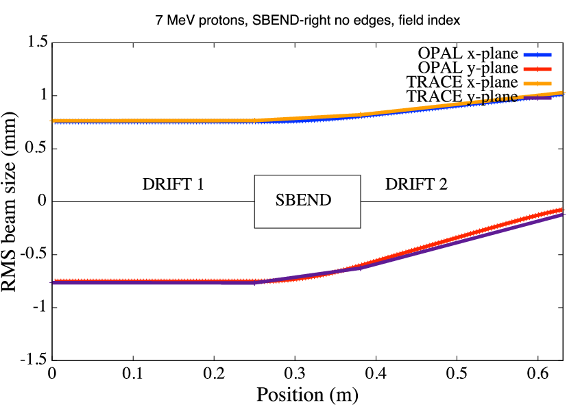
-
From TRACE 3D to OPAL-t
| Parameter | Trace 3D | OPAL-t |
|---|---|---|
Bend card |
8 |
|
Angle |
Input parameter [deg] |
Input/Calc. parameter [rad] |
Magn. field |
Calculated. [T] |
Input/Calc parameter [T] |
Radius of curv. |
Input parameter [mm] |
Output information [m] |
Field-index |
Input parameter |
Input parameter |
Length |
Calculated [mm] |
Input/Calc parameter [m] |
Length type |
Effective |
Straight |
Edge card |
9 |
|
Edge angle |
Input parameter [deg] |
Input parameter [rad] |
Vertical gap |
9 |
|
Gap |
Total [mm] |
Total [m] |
Fringe field card |
9 |
FIELD MAP |
|
Default: 0.45 |
- |
|
Default: 2.8 |
- |
Bend direction |
Bend angle sign |
Coord. rotation |
Horiz. right |
Angle |
Angle |
Horiz. left |
Angle |
Angle |
Vertical bend |
Card 8, vf |
Coord. rotation |
1.1.12. Conclusion
-
TRACE 3D and TRANSPORT:
-
a perfect agreement has been found between these two codes in transversal envelope and emittance;
-
changing the TRANSPORT units, the input beam parameters, in terms of sigma-matrix coefficients, can directly be imported from TRACE 3D file.
-
-
TRACE 3D and OPAL-t:
-
a good agreement has been found between these two codes in case of sector bending magnet with and without edge angles;
-
the default magnetic field map seems not working properly if the field index is not zero
-
an improvement of the test map used is needed in order to match the TRACE 3D emittance see Figure [SBEND_FI_test].
-
1.2. Hard Edge Dipole Comparison with ELEGANT
1.2.1. OPAL Dipole
When defining a dipole (SBEND or RBEND) in OPAL, a fringe field
map which defines the range of the field and the Enge coefficients is
required. If no map is provided, the code uses a default map. Here is a
dipole definition using the default map:
      bend1: SBEND, ANGLE = bend_angle,
      E1 = 0, E2 = 0,
      FMAPFN = "1DPROFILE1-DEFAULT",
      ELEMEDGE = drift_before_bend,
      DESIGNENERGY = bend_energy,
      L = bend_length,
      WAKEF = FS_CSR_WAKE;
Please refer to Section [1DProfile1] for the definition of the field map
and the default map 1DPROFILE1-DEFAULT. It defines a fringe field that
extends to 10 cm away from a dipole edge in both directions and it has
both B_y and B_z components. This makes the
comparison between OPAL and other codes which uses a hard edge dipole
by default,cumbersome because one needs to carefully integrate thought
the fringe field region in OPAL in order to come up with the
integrated fringe field value (FINT in ELEGANT) that usually used by
these codes, e.g. the ELEGANT and the TRACE3D. So we need to find a
default map for the hard edge dipole in OPAL.
1.2.2. Map for Hard Edge Dipole
The proposed default map for a hard edge dipole can be:
1DProfile1  0  0  2
-0.00000001 0.0 0.00000001 3
-0.00000001 0.0 0.00000001 3
-99.9
-99.9
On the first line, the two zeros following 1DProfile1 are the orders
of the Enge coefficient for the entrance and exit edge of the dipole.
2 cm is the default dipole gap width. The second line
defines the fringe field region of the entrance edge of the dipole which
extends from -0.00000001 cm to
0.00000001 cm. The third line defines the same fringe
field region for the exit edge of the dipole. The 3s on
both line don’t mean anything, they are just placeholders. On the fourth
and fifth line, the zeroth order Enge coefficients for both edges are
given. Since they are large negative numbers, the field in the fringe
field region has no B_z component and its
B_y component is just like the field in the middle of the
dipole.
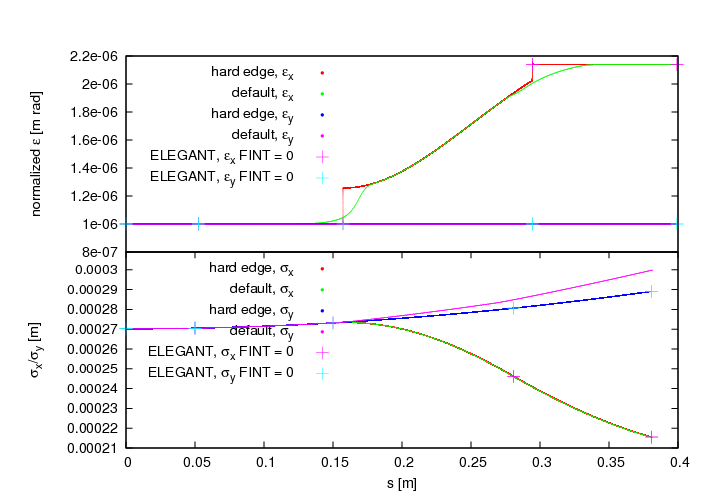
Figure [plot-compare-default] compares the emittances and beam sizes obtained by using the hard edge map, the default map and the ELEGANT. One can see that the results produced by the hard edge map match the ELEGANT results when FINT is set to zero.
1.2.3. Integration Time Step
When the hard edge map is used for a dipole, finer integration time step
is needed to ensure the accurate of the calculation.
Figure [plot-emit-dt] compares the normalized emittances generated using
the hard edge map in OPAL with varying time steps to those from the
ELEGANT. 0.01ps seems to be a optimal time step for the fringe field
region. To speed up the simulations, one can use larger time steps
outside the fringe field regions. In Figure [plot-emit-dt], one can
observe a discontinuity in the horizontal emittance when the hard edge
map is used in the calculation. This discontinuity comes from the fact
that OPAL emittance is calculated at an instant time. Once the beam or
part of the beam gets into the dipole, its P_x gets a kick
which will result in a sudden emittance change.
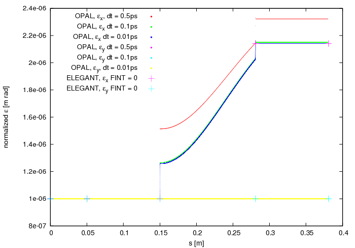
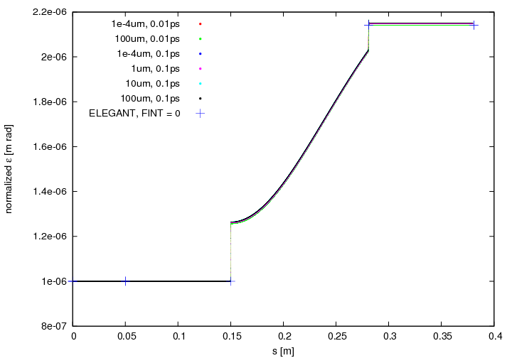
Figure [plot-fringe-size,plot-fringe-size-zoom] examine the effects of the fringe field range and the integration time step on the simulation accuracy. Figure [plot-fringe-size-zoom] is a zoom-in plot of Figure [plot-fringe-size]. We can conclude that the size of the integration time step has more influence on the accuracy of the simulation.

1.3. 1D CSR comparison with ELEGANT
1D-CSR wake function can now be used for the drift element by defining
its attribute WAKEF = FS_CSR_WAKE. In order to calculate the CSR
effect correctly, the drift has to follow a bending magnet whose CSR
calculation is also turned on.
      bend1: SBEND, ANGLE = bend_angle,
      E1 = 0, E2 = 0,
      FMAPFN = "1DPROFILE1-DEFAULT",
      ELEMEDGE = drift_before_bend,
      DESIGNENERGY = bend_energy,
      L = bend_length,
      WAKEF = FS_CSR_WAKE;
       drift1: DRIFT, L=0.4, ELEMEDGE = drift_before_bend +
       bend_length, WAKEF = FS_CSR_WAKE;
1.3.1. Benchmark
The OPAL dipoles all have fringe fields. When comparisons are done
between OPAL and ELEGANT [elegant] for example, one needs to
appropriately set the FINT attribute of the bending magnet in ELEGANT in
order to represent the field correctly. Although ELEGANT tracks in the
(x, x', y, y', s, \delta) phase space, where
\delta = \frac{\Delta p}{p_0} and p_0 is the
momentum of the reference particle, the watch point output beam
distributions from the ELEGANT are list in
(x, x', y, y', t, \beta\gamma). If one wants to compare
ELEGANT watch point output distribution to OPAL, unit conversion needs
to be performed, i.e.
\begin{aligned}
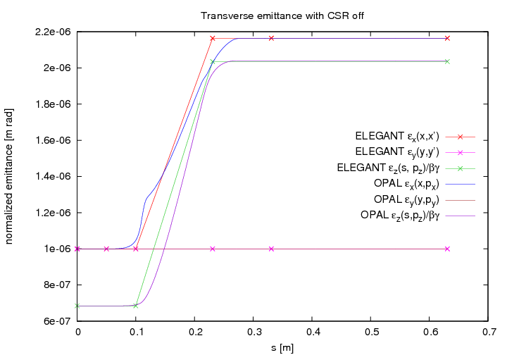
P_x &=& x'\beta\gamma, \\ P_y &=& y'\beta\gamma, \\ s &=& (\bar t-t)\beta c .\end{aligned}To benchmark the CSR effect, we set up a simple beamline with 0.1m drift
] 30 degree sbend latexmath:[ 0.4m drift. When the CSR
effect is turn off, Figure [plot-emit-csr-off] shows that the normalized
emittances calculated using both OPAL and ELEGANT agree. The emittance
values from OPAL are obtained from the .stat file, while for
ELEGANT, the transverse emittances are obtained from the sigma output
file (enx, and eny), the longitudinal emittance is calculated using the
watch point beam distribution output.
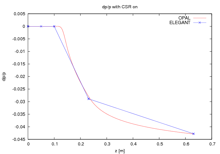
When CSR calculations are enabled for both the bending magnet and the
following drift, Figure [plot-dpp-csr-on] shows the average
\delta or \frac{\Delta p}{p} change along
the beam line, and Figure [plot-emit-csr-on] compares the normalized
transverse and longitudinal emittances obtained by these two codes. The
average \frac{\Delta p}{p} can be found in the centroid
output file (Cdelta) from ELEGANT, while in OPAL, one can calculate it
using
\frac{\Delta p}{p} = \frac{1}{\beta^2}\frac{\Delta \overline{E}}{\overline{E}+mc^2},
where \Delta \overline{E} is the average kinetic energy
from the .stat output file.
\frac{\Delta p}{p} in Elegant and OPAL
In the drift space following the bending magnet, the CSR effects are
calculated using Stupakov’s algorithm with the same setting in both
codes. The average fractional momentum change
\frac{\Delta p}{p} and the longitudinal emittance show
good agreements between these codes. However, they produce different
horizontal emittances as indicated in Figure [plot-emit-csr-on].
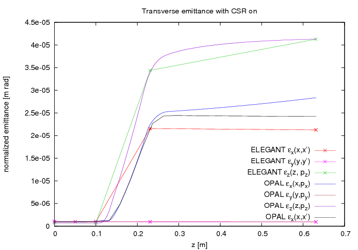
One important effect to notice is that in the drift space following the
bending magnet, the normalized emittance
\epsilon_x(x, P_x) output by OPAL keeps increasing while
the trace-like emittance \epsilon_x(x, x') calculated by
ELEGANT does not. This can be explained by the fact that with a
relatively large energy spread (about 3\% at the end of
the dipole due to CSR), an correlation between transverse position and
energy can build up in a drift thereby induce emittance growth. However,
this effect can only be observed in the normalized emittance calculated
with
\epsilon_x(x, P_x) = \sqrt{\langle x^2 \rangle \langle P_x^2\rangle - \langle xP_x \rangle^2}
where P_x = \beta\gamma x', not the trace-like emittance
which is calculated as
\epsilon_x (x, x') = \beta \gamma \sqrt{\langle x^2 \rangle \langle x' {}^{2} \rangle - \langle xx' \rangle^2}
[prstab2003]. In Figure [plot-emit-csr-on], a trace-like horizontal
emittance is also calcualted for the OPAL output beam distributions.
Like the ELEGANT result, this trace-like emittance doesn’t grow in the
drift. However, their differences come from the ELEGANT’s lack of CSR
effect in the fringe field region.
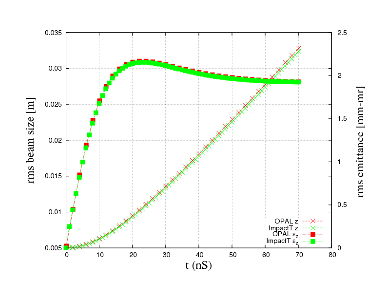
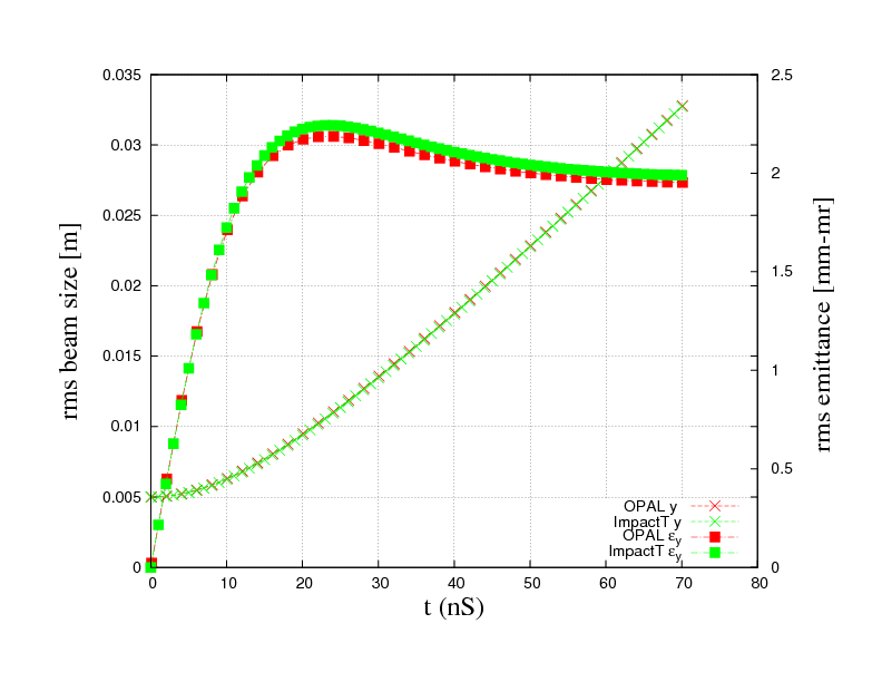
1.4. OPAL & Impact-t
This benchmark compares rms quantities such as beam size and emittance
of OPAL and Impact-t [qiang2005, qiang2006-1, qiang2006-2]. A cold
10mA H+ bunch is expanding in a 1m drift space. A Gaussian distribution,
with a cut at 4 \sigma is used. The charge is computed by
assuming a 1MHz structure i.e.
Q_{\text{tot}}=\frac{I}{\nu_{\text{rf}}}. For the
simulation we use a grid with 16^{3} grid point and open
boundary condition. The number of macro particles is
N_{\text{p}} = 10^{5}.
1.4.1. OPAL Input
OPTION, ECHO = FALSE, PSDUMPFREQ = 10,
STATDUMPFREQ = 10, REPARTFREQ = 1000,
PSDUMPLOCALFRAME = FALSE, VERSION=10600;

TITLE, string="Gaussian bunch drift test";

REAL Edes    = 0.001;        // GeV
REAL CURRENT = 0.01;  // A

REAL gamma=(Edes+PMASS)/PMASS;
REAL beta=sqrt(1-(1/gamma^2));
REAL gambet=gamma*beta;
REAL P0 = gamma*beta*PMASS;

D1: DRIFT, ELEMEDGE = 0.0, L = 1.0;

L1: LINE = (D1);

Fs1: FIELDSOLVER, FSTYPE = FFT, MX = 16, MY = 16, MT = 16, BBOXINCR=0.1;

Dist1: DISTRIBUTION, TYPE = GAUSS,
       OFFSETX = 0.0, OFFSETY = 0.0, OFFSETZ = 15.0e-3,
       SIGMAX = 5.0e-3, SIGMAY = 5.0e-3, SIGMAZ = 5.0e-3,
       OFFSETPX = 0.0, OFFSETPY = 0.0, OFFSETPZ = 0.0,
       SIGMAPX = 0.0 , SIGMAPY = 0.0 , SIGMAPZ = 0.0 ,
       CORRX = 0.0, CORRY = 0.0, CORRZ = 0.0,
       CUTOFFX = 4.0, CUTOFFY = 4.0, CUTOFFLONG = 4.0;

Beam1: BEAM, PARTICLE = PROTON, CHARGE = 1.0, BFREQ = 1.0, PC = P0,
               NPART = 1E5, BCURRENT = CURRENT, FIELDSOLVER = Fs1;

SELECT, LINE = L1;

TRACK, LINE = L1, BEAM = Beam1, MAXSTEPS = 1000, ZSTOP = 1.0, DT = 1.0e-10;
 RUN, METHOD = "PARALLEL-T", BEAM = Beam1, FIELDSOLVER = Fs1, DISTRIBUTION = Dist1;
ENDTRACK;
STOP;
1.4.2. Impact-t Input
!Welcome to Impact-t input file.
!All comment lines start with "!" as the first character of the line.
! col row
1 1
!
! information needed by the integrator:
! step-size, number of steps, and number of bunches/bins (??)
!
!   dt    Ntstep  Nbunch
1.0e-10   700     1
!
! phase-space dimension, number of particles, a series of flags
! that set the type of integrator, error study, diagnostics, and
! image charge, and the cutoff distance for the image charge
!
! PSdim  Nptcl   integF  errF  diagF  imchgF  imgCutOff (m)
6 100000  1 0 1 0 0.016
!
! information about mesh: number of points in x, y, and z, type
! of boundary conditions, transverse aperture size (m),
! and longitudinal domain size (m)
!
!  Nx  Ny  Nz  bcF   Rx    Ry    Lz
16 16 16 1 0.15 0.15 1.0e5
!
!
! distribution type number (2 == Gauss), restart flag, space-charge substep
! flag, number of emission steps, and max emission time
!
! distType  restartF  substepF  Nemission  Temission
2           0         0         -1          0.0
!
!  sig*   sigp*  mu*p*  *scale  p*scale  xmu*      xmu*
!
0.005 0.0 0.0  1. 1. 0.0 0.0
0.005 0.0 0.0  1. 1. 0.0 0.0
0.005 0.0 0.0  1. 1. 0.0 0.0462
!
! information about the beam: current, kinetic energy, particle
! rest energy, particle charge, scale frequency, and initial cavity phase
!
! I/A   Ek/eV     Mc2/eV          Q/e  freq/Hz  phs/rad
0.010   1.0e6     938.271998e+06  1.0  1.0e6      0.0
!
!
! ======= machine description starts here =======
! the following lines, which must each be terminated with a '/',
! describe one beam-line element per line; the basic structure is
! element length, ???, ???, element type, and then a sequence of
! at most 24 numbers describing the element properties
!   0  drift tube    2      zedge radius
!   1  quadrupole    9      zedge, quad grad, fileID,
!                             radius, alignment error x, y
!                             rotation error x, y, z
! L/m  N/A N/A  type  location of starting edge  v1  <B0><B0><B0>  v23 /
1.0    0   0    0    0.0                           0.5            /
1.4.3. Results
A good agreement is shown in the
Figure [plot-opal-impact1,plot-opal-impact2]. This proves to some extend
the compatibility of the space charge solvers of OPAL and Impact-t.
Impact-t and OPAL
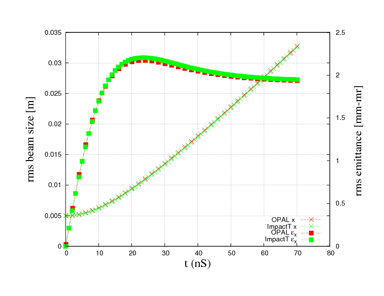
Impact-t and OPAL