1. OPAL-t
1.1. Introduction
OPAL-t is a fully three-dimensional program to track in time, relativistic particles taking into account space charge forces, self-consistently in the electrostatic approximation, and short-range longitudinal and transverse wake fields. OPAL-t is one of the few codes that is implemented using a parallel programming paradigm from the ground up. This makes OPAL-t indispensable for high statistics simulations of various kinds of existing and new accelerators. It has a comprehensive set of beamline elements, and furthermore allows arbitrary overlap of their fields, which gives OPAL-t a capability to model both the standing wave structure and traveling wave structure. Beside IMPACT-T it is the only code making use of space charge solvers based on an integrated Green [qiang2005, qiang2006-1,qiang2006-2] function to efficiently and accurately treat beams with large aspect ratio, and a shifted Green function to efficiently treat image charge effects of a cathode [fubiani2006, qiang2005, qiang2006-1,qiang2006-2]. For simulations of particles sources i.e. electron guns OPAL-t uses the technique of energy binning in the electrostatic space charge calculation to model beams with large energy spread. In the very near future a parallel Multigrid solver taking into account the exact geometry will be implemented.
1.2. Variables in OPAL-t
OPAL-t uses the following canonical variables to describe the motion of particles. The physical units are listed in square brackets.
- X
-
Horizontal position
xof a particle relative to the axis of the element [m]. - PX
-
\beta_x\gammaHorizontal canonical momentum [1]. - Y
-
Horizontal position
yof a particle relative to the axis of the element [m]. - PY
-
\beta_y\gammaHorizontal canonical momentum [1]. - Z
-
Longitudinal position
zof a particle in floor co-ordinates [m]. - PZ
-
\beta_z\gammaLongitudinal canonical momentum [1].
The independent variable is t [s].
1.3. Integration of the Equation of Motion
OPAL-t integrates the relativistic Lorentz equation
\frac{\mathrm{d}\gamma\mathbf{v}}{\mathrm{d}t} = \frac{q}{m}[\mathbf{E}_{ext} + \mathbf{E}_{sc} + \mathbf{v} \times (\mathbf{B}_{ext} + \mathbf{B}_{sc})]where \gamma is the relativistic factor, q
is the charge, and m is the rest mass of the particle.
\mathbf{E} and \mathbf{B} are abbreviations
for the electric field \mathbf{E}(\mathbf{x},t) and
magnetic field \mathbf{B}(\mathbf{x},t). To update the
positions and momenta OPAL-t uses the Boris-Buneman algorithm
[langdon].
1.4. Positioning of Elements
Since OPAL version 2.0 of OPAL elements can be placed in space using
3D coordinates X, Y, Z, THETA, PHI and PSI, see
Section [Element:common]. The old notation using ELEMEDGE is still
supported. OPAL-t then computes the position in 3D using ELEMDGE,
ANGLE and DESIGNENERGY. It assumes that the trajectory consists of
straight lines and segments of circles. Fringe fields are ignored. For
cases where these simplifications aren’t justifiable the user should use
3D positioning. For a simple switchover OPAL writes a file _3D.opal
where all elements are placed in 3D.
Beamlines containing guns should be supplemented with the element
SOURCE. This allows OPAL to distinguish the cases and adjust the
initial energy of the reference particle.
Prior to OPAL version 2.0 elements needed only a defined length. The transverse extent was not defined for elements except when combined with 2D or 3D field maps. An aperture had to be designed to give elements a limited extent in transverse direction since elements now can be placed freely in three-dimensional space. See Section [Element:common] for how to define an aperture.
1.5. Coordinate Systems
The motion of a charged particle in an accelerator can be described by
relativistic Hamilton mechanics. A particular motion is that of the
reference particle, having the central energy and traveling on the
so-called reference trajectory. Motion of a particle close to this
fictitious reference particle can be described by linearized equations
for the displacement of the particle under study, relative to the
reference particle. In OPAL-t, the time t is used as
independent variable instead of the path length s. The
relation between them can be expressed as
\frac{\mathrm{d}}{\mathrm{d} t} = \frac{\mathrm{d}}{\mathrm{d}\mathbf{s}}\frac{\mathrm{d}\mathbf{s}}{\mathrm{d} t} = \mathbf{\beta}c\frac{\mathrm{d}}{\mathrm{d}\mathbf{s}}.Global Cartesian Coordinate System
We define the global cartesian coordinate system, also known as floor
coordinate system with K, a point in this coordinate
system is denoted by (X, Y, Z) \in K. In Figure [KS1] of
the accelerator is uniquely defined by the sequence of physical elements
in K. The beam elements are numbered
e_0, \ldots , e_i, \ldots e_n.
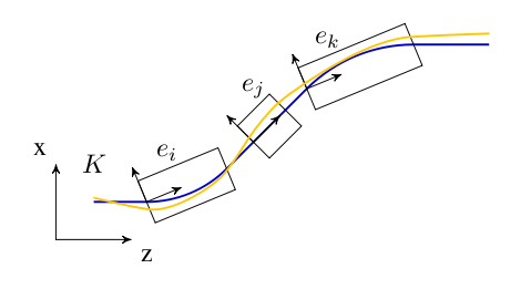
Local Cartesian Coordinate System
A local coordinate system K'_i is attached to each element
e_i. This is simply a frame in which (0,0,0)
is at the entrance of each element. For an illustration see
Figure [KS1]. The local reference system
(x, y, z) \in K'_n may thus be referred to a global
Cartesian coordinate system (X, Y, Z) \in K.
The local coordinates (x_i, y_i, z_i) at element
e_i with respect to the global coordinates
(X, Y, Z) are defined by three displacements
(X_i, Y_i, Z_i) and three angles
(\Theta_i, \Phi_i, \Psi_i).
\Psi is the roll angle about the global
Z-axis. \Phi is the pitch angle about the
global Y-axis. Lastly, \Theta is the yaw
angle about the global X-axis. All three angles form
right-handed screws with their corresponding axes. The angles
(\Theta,\Phi,\Psi) are the Tait-Bryan angles
[bib:tait-bryan].
The displacement is described by a vector \mathbf{v} and
the orientation by a unitary matrix \mathcal{W}. The
column vectors of \mathcal{W} are unit vectors spanning
the local coordinate axes in the order (x, y, z).
\mathbf{v} and \mathcal{W} have the values:
\mathbf{v} =\left(\begin{array}{c}
    X \\
    Y \\
    Z
  \end{array}\right),
\qquad
\mathcal{W}=\mathcal{S}\mathcal{T}\mathcal{U}
where
\mathcal{S}=\left(\begin{array}{ccc}
    \cos\Theta &  0 &  \sin\Theta \\
    0         &  1 &   0 \\
    -\sin\Theta &  0 &  \cos\Theta
  \end{array}\right),
\quad
\mathcal{T}=\left(\begin{array}{ccc}
    1 &  0        &  0 \\
    0 &  \cos\Phi &  \sin\Phi \\
    0 & -\sin\Phi &  \cos\Phi
  \end{array}\right),
\quad
\mathcal{U}=\left(\begin{array}{ccc}
    \cos\Psi & -\sin\Psi &  0 \\
    \sin\Psi &  \cos\Psi &  0 \\
    0        &  0        &  1
  \end{array}\right).
We take the vector \mathbf{r}_i to be the displacement and
the matrix \mathcal{S}_i to be the rotation of the local
reference system at the exit of the element i with respect
to the entrance of that element.
Denoting with i a beam line element, one can compute
\mathbf{v}_i and \mathcal{W}_i by the
recurrence relations
\mathbf{v}_i = \mathcal{W}_{i-1}\mathbf{r}_i + \mathbf{v}_{i-1}, \qquad
\mathcal{W}_i = \mathcal{W}_{i-1}\mathcal{S}_i,
where
\mathbf{v}_0 corresponds to the origin of the LINE and
\mathcal{W}_0 to its orientation. In OPAL-t they can be
defined using either X, Y, Z, THETA, PHI and PSI or ORIGIN
and ORIENTATION, see Section [line:simple].
Space Charge Coordinate System
In order to calculate space charge in the electrostatic approximation,
we introduce a co-moving coordinate system K_{\text{sc}},
in which the origin coincides with the mean position of the particles
and the mean momentum is parallel to the z-axis.
Curvilinear Coordinate System
In order to compute statistics of the particle ensemble,
K_s is introduced. The accompanying tripod (Dreibein) of
the reference orbit spans a local curvilinear right handed system
(x,y,s). The local s-axis is the tangent to
the reference orbit. The two other axes are perpendicular to the
reference orbit and are labelled x (in the bend plane)
and y (perpendicular to the bend plane).
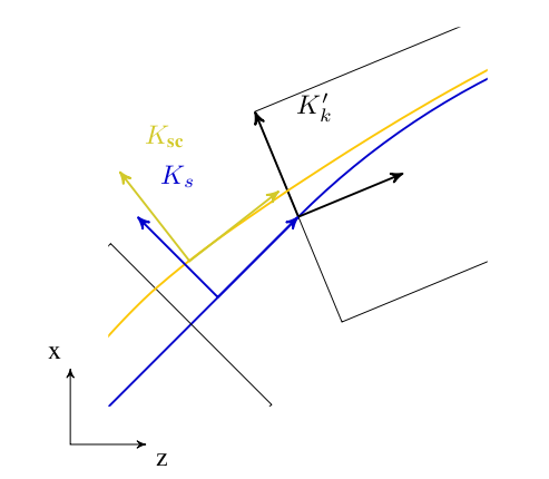 K_\text{sc} and
 K_s">
Both coordinate systems are described in Figure [KS2].
1.5.5. Design or Reference Orbit
The reference orbit consists of a series of straight sections and circular arcs and is computed by the Orbit Threader i.e. deduced from the element placement in the floor coordinate system.
1.5.6. Compatibility Mode
To facilitate the change for users we will provide a compatibility mode.
The idea is that the user does not have to change the input file.
Instead OPAL-t will compute the positions of the elements. For this it
uses the bend angle and chord length of the dipoles and the position of
the elements along the trajectory. The user can choose whether effects
due to fringe fields are considered when computing the path length of
dipoles or not. The option to toggle OPAL-t’s behavior is called
IDEALIZED. OPAL-t assumes per default that provided ELEMEDGE for
elements downstream of a dipole are computed without any effects due to
fringe fields.
Elements that overlap with the fields of a dipole have to be handled separately by the user to position them in 3D.
We split the positioning of the elements into two steps. In a first step we compute the positions of the dipoles. Here we assume that their fields don’t overlap. In a second step we can then compute the positions and orientations of all other elements.
The accuracy of this method is good for all elements except for those that overlap with the field of a dipole.
1.5.7. Orbit Threader and Autophasing
The OrbitThreader integrates a design particle through the lattice and
setups up a multi map structure (IndexMap). Furthermore when the
reference particle hits an rf-structure for the first time then it
auto-phases the rf-structure, see Appendix [autophasing]. The multi map
structure speeds up the search for elements that influence the particles
at a given position in 3D space by minimizing the looping over elements
when integrating an ensemble of particles. For each time step,
IndexMap returns a set of elements
\mathcal{S}_{\text{e}} \subset {e_0 \ldots e_n} in case of
the example given in Figure [KS1]. An implicit drift is modelled as an
empty set \emptyset.
1.5.8. Flow Diagram of OPAL-t
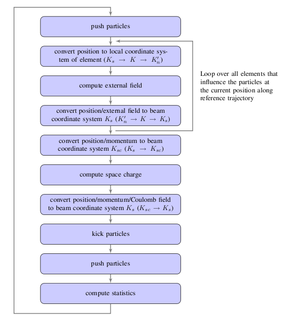
A regular time step in OPAL-t is sketched in
Figure [OPALTSchemeSimple]. In order to compute the coordinate system
transformation from the reference coordinate system K_s to
the local coordinate systems K'_n we join the
transformation from floor coordinate system K to
K'_n to the transformation from K_s to
K. All computations of rotations which are involved in the
computation of coordinate system transformations are performed using
quaternions. The resulting quaternions are then converted to the
appropriate matrix representation before applying the rotation operation
onto the particle positions and momenta.
As can be seen from Figure [OPALTSchemeSimple] the integration of the trajectories of the particles are integrated and the computation of the statistics of the six-dimensional phase space are performed in the reference coordinate system.
1.6. Output
In addition to the progress report that OPAL-t writes to the standard output (stdout) it also writes different files for various purposes.
1.6.1. <input_file_name >.stat
This file is used to log the statistical properties of the bunch in the
ASCII variant of the SDDS format [bib:borland1995]. It can be viewed
with the SDDS Tools [bib:borland2016] or GNUPLOT. The frequency with
which the statistics are computed and written to file can be controlled
With the option STATDUMPFREQ. The information that is stored are found
in the following table.
| Column Nr. | Name | Units | Meaning |
|---|---|---|---|
1 |
t |
ns |
Time |
2 |
s |
m |
Path length |
3 |
numParticles |
1 |
Number of macro particles |
4 |
charge |
C |
Charge of bunch |
5 |
energy |
MeV |
Mean energy of bunch |
6 |
rms_x |
m |
Standard deviation of x-component of particles positions |
7 |
rms_y |
m |
Standard deviation of y-component of particles positions |
8 |
rms_s |
m |
Standard deviation of s-component of particles positions |
9 |
rms_px |
1 |
Standard deviation of x-component of particles normalized momenta |
10 |
rms_py |
1 |
Standard deviation of y-component of particles normalized momenta |
11 |
rms_ps |
1 |
Standard deviation of s-component of particles normalized momenta |
12 |
emit_x |
mrad |
X-component of normalized emittance |
13 |
emit_y |
mrad |
Y-component of normalized emittance |
14 |
emit_s |
mrad |
S-component of normalized emittance |
15 |
mean_x |
m |
X-component of mean position relative to reference particle |
16 |
mean_y |
m |
Y-component of mean position relative to reference particle |
17 |
mean_s |
m |
S-component of mean position relative to reference particle |
18 |
ref_x |
m |
X-component of reference particle in floor coordinate system |
19 |
ref_y |
m |
Y-component of reference particle in floor coordinate system |
20 |
ref_z |
m |
Z-component of reference particle in floor coordinate system |
21 |
ref_px |
1 |
X-component of normalized momentum of reference particle in floor coordinate system |
22 |
ref_py |
1 |
Y-component of normalized momentum of reference particle in floor coordinate system |
23 |
ref_pz |
1 |
Z-component of normalized momentum of reference particle in floor coordinate system |
24 |
max_x |
m |
Max beamsize in x-direction |
25 |
max_y |
m |
Max beamsize in y-direction |
26 |
max_s |
m |
Max beamsize in s-direction |
27 |
xpx |
1 |
Correlation between x-components of positions and momenta |
28 |
ypy |
1 |
Correlation between y-components of positions and momenta |
29 |
zpz |
1 |
Correlation between s-components of positions and momenta |
30 |
Dx |
m |
Dispersion in x-direction |
31 |
DDx |
1 |
Derivative of dispersion in x-direction |
32 |
Dy |
m |
Dispersion in y-direction |
33 |
DDy |
1 |
Derivative of dispersion in y-direction |
34 |
Bx_ref |
T |
X-component of magnetic field at reference particle |
35 |
By_ref |
T |
Y-component of magnetic field at reference particle |
36 |
Bz_ref |
T |
Z-component of magnetic field at reference particle |
37 |
Ex_ref |
MVm^-1 |
X-component of electric field at reference particle |
38 |
Ey_ref |
MVm^-1 |
Y-component of electric field at reference particle |
39 |
Ez_ref |
MVm^-1 |
Z-component of electric field at reference particle |
40 |
dE |
MeV |
Energy spread of the bunch |
41 |
dt |
ns |
Size of time step |
42 |
partsOutside |
1 |
Number of particles outside
|
43 |
R0_x |
m |
X-component of position of particle with ID 0 (only when run serial) |
44 |
R0_y |
m |
Y-component of position of particle with ID 0 (only when run serial) |
45 |
R0_s |
m |
S-component of position of particle with ID 0 (only when run serial) |
46 |
P0_x |
m |
X-component of momentum of particle with ID 0 (only when run serial) |
47 |
P0_y |
m |
Y-component of momentum of particle with ID 0 (only when run serial) |
48 |
P0_s |
m |
S-component of momentum of particle with ID 0 (only when run serial) |
1.6.2. data/<input_file_name >_Monitors.stat
OPAL-t computes the statistics of the bunch for every MONITOR that
it passes. The information that is written can be found in the following
table.
| Column Nr. | Name | Units | Meaning |
|---|---|---|---|
1 |
name |
a string |
Name of the monitor |
2 |
s |
m |
Position of the monitor in path length |
3 |
t |
ns |
Time at which the reference particle pass |
4 |
numParticles |
1 |
Number of macro particles |
5 |
rms_x |
m |
Standard deviation of the x-component of the particles positions |
6 |
rms_y |
m |
Standard deviation of the y-component of the particles positions |
7 |
rms_s |
m |
Standard deviation of the s-component of the particles
positions (only nonvanishing when type of |
8 |
rms_t |
ns |
Standard deviation of the passage time of the particles
(zero if type is of |
9 |
rms_px |
1 |
Standard deviation of the x-component of the particles momenta |
10 |
rms_py |
1 |
Standard deviation of the y-component of the particles momenta |
11 |
rms_ps |
1 |
Standard deviation of the s-component of the particles momenta |
12 |
emit_x |
mrad |
X-component of the normalized emittance |
13 |
emit_y |
mrad |
Y-component of the normalized emittance |
14 |
emit_s |
mrad |
S-component of the normalized emittance |
15 |
mean_x |
m |
X-component of mean position relative to reference particle |
16 |
mean_y |
m |
Y-component of mean position relative to reference particle |
17 |
mean_s |
m |
S-component of mean position relative to reference particle |
18 |
mean_t |
ns |
Mean time at which the particles pass |
19 |
ref_x |
m |
X-component of reference particle in floor coordinate system |
20 |
ref_y |
m |
Y-component of reference particle in floor coordinate system |
21 |
ref_z |
m |
Z-component of reference particle in floor coordinate system |
22 |
ref_px |
1 |
X-component of normalized momentum of reference particle in floor coordinate system |
23 |
ref_py |
1 |
Y-component of normalized momentum of reference particle in floor coordinate system |
24 |
ref_pz |
1 |
Z-component of normalized momentum of reference particle in floor coordinate system |
25 |
max_x |
m |
Max beamsize in x-direction |
26 |
max_y |
m |
Max beamsize in y-direction |
27 |
max_s |
m |
Max beamsize in s-direction |
28 |
xpx |
1 |
Correlation between x-components of positions and momenta |
29 |
ypy |
1 |
Correlation between y-components of positions and momenta |
40 |
zpz |
1 |
Correlation between s-components of positions and momenta |
1.6.3. data/<input_file_name >_3D.opal
OPAL-t copies the input file into this file and replaces all
occurrences of ELEMEDGE with the corresponding position using X,
Y, Z, THETA, PHI and PSI.
1.6.4. data/<input_file_name >_ElementPositions.txt
OPAL-t stores for every element the position of the entrance and the
exit. Additionally the reference trajectory inside dipoles is stored. On
the first column the name of the element is written prefixed with
BEGIN: '', END: '' and ``MID: '' respectively. The remaining columns
store the z-component then the x-component and finally the y-component
of the position in floor coordinates.
1.6.5. data/<input_file_name >_ElementPositions.py
This Python script can be used to generate visualizations of the beam line in different formats. Beside an ASCII file that can be printed using GNUPLOT a VTK file and an HTML file can be generated. The VTK file can then be opened in e.g. ParaView [paraview,bib:paraview] or VisIt [bib:visit]. The HTML file can be opened in any modern web browser. Both the VTK and the HTML output are three-dimensional. For the ASCII format on the other hand you have provide the normal of a plane onto which the beam line is projected.
The script is not directly executable. Instead one has to pass it as
argument to python:
python myinput_ElementPositions.py --export-web
The following arguments can be passed
-
-hor--helpfor a short help -
--export-vtkto export to the VTK format -
--export-webto export for the web -
--project-to-plane x y zto project the beam line to the plane with the normal with the componentsx,yandz
1.6.6. data/<input_file_name >_ElementPositions.stat
This file can be used when plotting the statistics of the bunch to indicate the positions of the magnets. It is written in the SDDS format. The information that is written can be found in the following table.
| Column Nr. | Name | Units | Meaning |
|---|---|---|---|
1 |
s |
m |
The position in path length |
2 |
dipole |
Whether the field of a dipole is present |
|
3 |
quadrupole |
1 |
Whether the field of a quadrupole is present |
4 |
sextupole |
Whether the field of a sextupole is present |
|
5 |
octupole |
Whether the field of a octupole is present |
|
6 |
decapole |
1 |
Whether the field of a decapole is present |
7 |
multipole |
1 |
Whether the field of a general multipole is present |
8 |
solenoid |
1 |
Whether the field of a solenoid is present |
9 |
rfcavity |
|
Whether the field of a cavity is present |
10 |
monitor |
1 |
Whether a monitor is present |
11 |
element_names |
a string |
The names of the elements that are present |
1.6.7. data/<input_file_name >_DesignPath.dat
The trajectory of the reference particle is stored in this ASCII file. The content of the columns are listed in the following table.
| Column Nr. | Units | Meaning | |
|---|---|---|---|
1 |
m |
Position in path length |
|
2 |
m |
X-component of position in floor coordinates |
|
3 |
m |
Y-component of position in floor coordinates |
|
4 |
m |
Z-component of position in floor coordinates |
|
5 |
1 |
X-component of momentum in floor coordinates |
|
6 |
1 |
Y-component of momentum in floor coordinates |
|
7 |
1 |
Z-component of momentum in floor coordinates |
|
8 |
MV m^-1 |
X-component of electric field at position |
|
9 |
MV m^-1 |
Y-component of electric field at position |
|
10 |
MV m^-1 |
Z-component of electric field at position |
|
11 |
T |
X-component of magnetic field at position |
|
12 |
T |
Y-component of magnetic field at position |
|
13 |
T |
Z-component of magnetic field at position |
|
14 |
MeV |
Kinetic energy |
|
15 |
s |
Time |
1.7. Multiple Species
In the present version only one particle species can be defined see Chapter [beam], however due to the underlying general structure, the implementation of a true multi species version of OPAL should be simple to accomplish.
1.8. Multipoles in different Coordinate systems
In the following sections there are three models presented for the fringe field of a multipole. The first one deals with a straight multipole, while the second one treats a curved multipole, both starting with a power expansion for the magnetic field. The last model tries to be different by starting with a more compact functional form of the field which is then adapted to straight and curved geometries.
1.8.1. Fringe field models
(for a straight multipole)
Most accelerator modeling codes use the hard-edge model for magnets - constant Hamiltonian. Real magnets always have a smooth transition at the edges - fringe fields. To obtain a multipole description of a field we can apply the theory of analytic functions.
\begin{aligned}
        \nabla \cdot \mathbf{B} & = 0 \Rightarrow \exists \quad \mathbf{A} \quad \text{with} \quad \mathbf{B} = \nabla \times \mathbf{A} \\
        \nabla \times \mathbf{B} & = 0 \Rightarrow \exists \quad V \quad \text{with} \quad \mathbf{B} = - \nabla V
    \end{aligned}
Assuming that A has only a non-zero
component A_s we get
\begin{aligned}
        B_x & = - \frac{\partial V}{\partial x} = \frac{\partial A_s}{\partial y} \\
        B_y & = - \frac{\partial V}{\partial y} = - \frac{\partial A_s}{\partial x}
    \end{aligned}
These equations are just the Cauchy-Riemann
conditions for an analytic function
\tilde{A} (z) = A_s (x, y) + i V(x,y). So the complex
potential is an analytic function and can be expanded as a power series
\tilde{A} (z) = \sum_{n=0}^{\infty} \kappa_n z^n, \quad \kappa_n = \lambda_n + i \mu_nwith \lambda_n, \mu_n being real constants. It is
practical to express the field in cylindrical coordinates
(r, \varphi, s)
\begin{aligned}
        x & = r \cos \varphi \quad y = r \sin \varphi  \\
        z^n & = r^n ( \cos n \varphi + i \sin n \varphi )
    \end{aligned}
From the real and imaginary parts of equation () we obtain
\begin{aligned}
        V(r, \varphi) & = \sum_{n=0}^{\infty} r^n ( \mu_n \cos n \varphi + \lambda_n \sin n \varphi ) \\
        A_s (r, \varphi) & = \sum_{n=0}^{\infty} r^n ( \lambda_n \cos n \varphi - \mu_n \sin n \varphi )
    \end{aligned}
Taking the gradient of -V(r, \varphi)
we obtain the multipole expansion of the azimuthal and radial field
components, respectively
\begin{aligned}
        B_{\varphi} & = - \frac{1}{r} \frac{\partial V}{\partial \varphi} = - \sum_{n=0}^{\infty} n r^{n-1} ( \lambda_n \cos n \varphi - \mu_n \sin n \varphi ) \\
        B_r & = - \frac{\partial V}{\partial r} = - \sum_{n=0}^{\infty} n r^{n-1} ( \mu_n \cos n \varphi + \lambda_n \sin n \varphi )
    \end{aligned}
Furthermore, we introduce the normal multipole
coefficient b_n and skew coefficient a_n
defined with the reference radius r_0 and the magnitude of
the field at this radius B_0 (these coefficients can be a
function of s in a more general case as it is presented further on).
b_n = - \frac{n \lambda_n}{B_0} r_0^{n-1} \qquad a_n = \frac{n \mu_n}{B_0} r_0^{n-1}\begin{aligned}
B_{\varphi}(r, \varphi) & = B_0 \sum_{n=1}^{\infty} ( b_n \cos n \varphi+ a_n \sin n \varphi ) \left( \frac{r}{r_0} \right) ^{n-1} \\
B_r (r, \varphi) & = B_0 \sum_{n=1}^{\infty} ( -a_n \cos n \varphi+ b_n \sin n \varphi ) \left( \frac{r}{r_0} \right) ^{n-1}
\end{aligned}To obtain a model for the fringe field of a straight multipole, a proposed starting solution for a non-skew magnetic field is
\begin{aligned}
        V & = \sum_{n=1}^{\infty} V_n (r,z) \sin n \varphi \\
        V_n & = \sum_{k=0}^{\infty} C_{n,k}(z) r^{n+2k}
    \end{aligned}
It is straightforward to derive a relation between coefficients
\nabla ^2 V = 0 \Rightarrow \frac{1}{r} \frac{\partial}{\partial r} \left( r \frac{\partial V_n}{\partial r} \right) + \frac{\partial^2 V_n}{\partial z^2} = \frac{n^2 V_n}{r^2} = 0V_n = \sum_{k=0}^{\infty} C_{n,k}(z) r^{n+2k}\Rightarrow \sum_{k=0}^{\infty} \left[ r^{n+2(k-1)} \left[ (n+2k)^2 - n^2 \right] C_{n,k}(z) + r^{n+2k} \frac{\partial^2 C_{n,k}(z)}{\partial z^2} \right] = 0By identifying the term in front of the same powers of r
we obtain the recurrence relation
C_{n,k}(z) = - \frac{1}{4k(n+k)} \frac{d^2 C_{n,k-1}} {dz^2}, k = 1,2, \ldotsThe solution of the recursion relation becomes
C_{n,k} (z) = (-1)^k \frac{n!}{2^{2k} k! (n+k)!} \frac{d^{2k} C_{n,0}(z)}{dz^{2k}}Therefore
V_n = - \left( \sum_{k=0}^{\infty} (-1)^{k+1} \frac{n!}{2^{2k} k! (n+k)!} C_{n, 0}^{(2k)}(z) r^{2k} \right) r^nThe transverse components of the field are
\begin{aligned}
        B_r & = \sum_{n=1}^{\infty} g_{rn} r^{n-1} \sin n \varphi \\
        B_{\varphi} & = \sum_{n=1}^{\infty} g_{\varphi n} r^{n-1} \cos n \varphi
    \end{aligned}
where the following gradients determine the entire
potential and can be deduced from the function C_{n,0}(z)
once the harmonic n is fixed.
\begin{aligned}
        g_{rn} (r,z) & = \sum_{k=0}^{\infty} (-1)^{k+1} \frac{n! (n+2k)}{2^{2k} k! (n+k)!} C_{n,0}^{(2k)}(z)r^{2k} \\
        g_{ \varphi n} (r,z) & = \sum_{k=0}^{\infty} (-1)^{k+1} \frac{n!n}{2^{2k} k! (n+k)!} C_{n,0}^{(2k)}(z)r^{2k}
    \end{aligned}
The z-directed component of the filed can be expressed in a similar form
\begin{aligned}
        B_z & = - \frac{\partial V}{\partial z} =  \sum_{n=1}^{\infty} g_{zn} r^n \sin n \varphi \\
        g_{zn} & = \sum_{k=0}^{\infty} (-1)^{k+1} \frac{n!}{2^{2k} k! (n+k)!} C_{n,0}^{2k+1} r^{2k}
    \end{aligned}
The gradient functions
g_{rn}, g_{\varphi n}, g_{zn} are obtained from
\begin{aligned}
        B_{r,n} & = - \frac{\partial V_n}{\partial r} \sin n \varphi = g_{rn} r^{n-1} \sin n \varphi \\
        B_{\varphi,n} & = - \frac{n}{r} V_n \cos n \varphi = g_{\varphi n} r^{n-1} \cos n \varphi \\
        B_{z,n} & = - \frac{\partial V_n}{\partial z} \sin n \varphi = g_{zn} r^{n} \sin n \varphi
    \end{aligned}
One preferred model to approximate the gradient profile on the central axis is the k-parameter Enge function
\begin{aligned}
        C_{n,0}(z) & = \frac{G_0}{1+exp[P(d(z))]}, \quad G_0 = \frac{B_0}{r_0^{n-1}} \\
        P(d) & = C_0 + C_1 \left( \frac{d}{\lambda} \right) + C_2 \left( \frac{d}{\lambda} \right)^2 + \ldots + C_{k-1} \left( \frac{d}{\lambda} \right)^{k-1}
    \end{aligned}
where d(z) is the distance to the
field boundary and \lambda characterizes the fringe field
length.
1.8.2. Fringe field of a curved multipole
(fixed radius)
We consider the Frenet-Serret coordinate system
( \hat{\mathbf{x}}, \hat{\mathbf{s}}, \hat{\mathbf{z}} )
with the radius of curvature \rho constant and the scale
factor h_s = 1 + x/ \rho. A conversion to these
coordinates implies that
\begin{aligned}
        \nabla \cdot \mathbf{B} & = \frac{1}{h_s} \left[ \frac{\partial (h_s B_x )}{\partial x} + \frac{\partial B_s}{\partial s} + \frac{\partial (h_s B_z )}{\partial z} \right] \\
        \nabla \times \mathbf{B} & = \frac{1}{h_s} \left[ \frac{\partial B_z}{\partial s} -  \frac{\partial (h_s B_s )}{\partial z} \right] \hat{\mathbf{x}} + \left[ \frac{\partial B_x}{\partial z} - \frac{\partial B_z}{\partial x} \right] \hat{\mathbf{s}} + \frac{1}{h_s} \left[ \frac{\partial (h_s B_s)}{\partial x} - \frac{\partial B_x}{\partial s} \right] \hat{\mathbf{z}} \nonumber
    \end{aligned}
To simplify the problem, consider multipoles with mid-plane symmetry, i.e.
b_z (z) = B_z (-z) \qquad B_x (z) = - B_x (-z) \qquad B_s (z) = - B_s (-z)The most general form of the expansion is
\begin{aligned}
         B_z & = \sum_{i,k=0}^{\infty} b_{i,k} x^i z^{2k}  \\
         B_x & = z \sum_{i,k=0}^{\infty} a_{i,k} x^i z^{2k} \\
         B_s & = z \sum_{i,k=0}^{\infty} c_{i,k} x^i z^{2k}
    \end{aligned}
Maxwell’s equations
\nabla \cdot \mathbf{B} = 0 and
\nabla \times \mathbf{B} = 0 in the above coordinates
yield
\frac{\partial}{\partial x} \left( (1+x/ \rho) B_x \right) + \frac{\partial B_s}{\partial s} + (1+x/ \rho) \frac{\partial B_z}{\partial z} = 0\begin{aligned}
\frac{\partial B_z}{\partial s} & = (1+x/ \rho) \frac{\partial B_s}{\partial z} \\
\frac{\partial B_x}{\partial z} & = \frac{\partial B_z}{\partial s} \\
\frac{\partial B_x}{\partial s} & = \frac{\partial}{\partial x} \left( (1+x/ \rho) B_s \right)
\end{aligned}The substitution of (1) into Maxwell’s equations allows for the derivation of recursion relations. ([eq:23]) gives
\sum_{i,k=0}^{\infty} a_{i,k} (2k+1) x^i z^{2k} = \sum_{i,k=0}^{\infty} b_{i,k} i x^{i-1} z^{2k}Equating the powers in x^i z^{2k}
a_{i,k} = \frac{i+1}{2k+1} b_{i+1,k}A similar result is obtained from ([eq:24])
\begin{aligned}
        \sum_{i,k=0}^{\infty} \partial_s b_{i,k} x^i z^{2k} & = \left( 1+ \frac{x}{\rho} \right) \sum_{i,k=0}^{\infty} c_{i,k} (2k+1) x^i z^{2k} \\
        \Rightarrow c_{i,k}  & + \frac{1}{\rho} c_{i-1,k} = \frac{1}{2k+1} \partial_s b_{i,k}
    \end{aligned}
The last equation from
\nabla \times \mathbf{B} = 0 should be consistent with the
two recursion relations obtained. ([eq:22]) implies
\sum_{i,k=0}^{\infty} \left[ \frac{i+1}{\rho} c_{i,k} x^i + c_{i,k} i x^{i-1} \right] z^{k+1} = \sum_{i,k=0}^{\infty} \partial_s a_{i,k} x^i z^{2k}\Rightarrow \frac{\partial_s a_{i,k}}{i+1} = \frac{1}{\rho} c_{i,k} + c_{i+1,k}This results follows directly from ([eq:11]) and ([eq:12]); therefore the relations are consistent. Furthermore, the last required relations is obtained from the divergence of B
\sum_{i,k=0}^{\infty} \left[ \frac{a_{i,k} x^i z^{2k+1}}{\rho} + i a_{i,k} x^{i-1} z^{2k+1} + \frac{i a_{i,k} x^i z^{2k+1}}{\rho} + \partial_s c_{i,k} x^i z^{2k+1} + 2kb_{i,k}x^i z^{2k-1} \right] = 0 \nonumber\Rightarrow \partial_s c_{i,k} + \frac{2(k+1)}{\rho} b_{i-1,k+1} + 2(k+1) b_{i,k+1} + \frac{1}{\rho} a_{i,k} + (i+1) a_{i+1,k} + \frac{1}{\rho} a_{i,k} = 0 \nonumberUsing the relation ([eq:11]) to replace the a coefficients
with b’s we arrive at
\partial_s c_{i,k} + \frac{(i+1)^2}{\rho (2k+1)} b_{i+1,k} + \frac{(i+1)(i+2)}{2k+1} b_{i+2,k} + \frac{2(k+1)}{\rho} b_{i-1,k+1} + 2(k+1) b_{i,k+1} = 0All the coefficients above can be determined recursively provided the
field B_z can be measured at the mid-plane in the form
B_z(z=0) = B_{0,0} + B_{1,0}x + B_{2,0} x^2 + B_{3,0} x^3 + \ldotswhere B_{i,0} are functions of s and they
can model the fringe field for each multipole term x^n. As
an example, for a dipole magnet, the B_{1,0} function can
be model as an Enge function or tanh.
1.8.3. Fringe field of a curved multipole
(variable radius of curvature)
The difference between this case and the above is that
\rho is now a function of s,
\rho(s). We can obtain the same result starting with the
same functional forms for the field (1). The
result of the previous section also holds in this case since no
derivative \frac{\partial}{\partial s} is applied to the
scale factor h_s. If the radius of curvature is set to be
proportional to the dipole filed observed by some reference particle
that stays in the centre of the dipole
rho (s) \propto B(z=0, x=0, s) = B_x (z=0,x=0) = b_{0,0}(s)1.8.4. Fringe field of a multipole
This is a different, more compact treatment The derivation is more clear if we gather the variables together in functions. We assume again mid-plane symmetry and that the z-component of the field in the mid-plane has the form
B_z (x, z=0, s) = T(x) S(s)where
T(s) is the transverse field profile and
S(s) is the fringe field. One of the requirements of the
symmetry is that B_z(z) = B_z(-z) which using a scalar
potential \psi requires
\frac{\partial \psi}{\partial z} to be an even function in
z. Therefore, \psi is an odd function in z and can be
written as
\psi = z f_0(x,s) + \frac{z^3}{3!} f_1(x,s) + \frac{z^5}{5!} f_3(x,s) + \ldotsThe given transverse profile requires that
f_0(x,s) = T(x)S(s), while \nabla^2 \psi = 0
follows from Maxwell’s equations as usual, more explicitly
\frac{\partial}{\partial x} \left( h_s \frac{\partial \psi}{\partial x} \right) + \frac{\partial}{\partial s} \left( \frac{1}{h_s} \frac{\partial \psi}{\partial s} \right) + \frac{\partial}{\partial z} \left( h_s \frac{\partial \psi}{\partial z} \right) = 0For a straight multipole h_s = 1. Laplace’s equation
becomes
\sum_{n=0} \frac{z^{2n+1}}{(2n+1)!} \left[ \partial_x^2 f_n(x,s) + \partial_s^2 f_n(x,s) \right] + \sum_{n=1} f_n(x,s) \frac{z^{n-1}}{(n-1)!} = 0By equating powers of z we obtain the recursion relation
f_{n+1}(x,s) = - \left( \partial_x^2 + \partial_s^2 \right) f_n(x,s)The general expression for any f_n(x,s) is then obtained
from the mid-plane field by
\begin{aligned}
        f_n(x,s) & = (-1)^n \left( \partial_x^2 + \partial_s^2 \right)^n f_0(x,s) \\
        f_n(x,s) & = (-1)^n \sum_{i=0}^n \binom{n}{i}T^{(2i)}(x) S^{(2n-2i)}(s)
    \end{aligned}
For a curved multipole of constant radius
h_s = 1 + \frac{x}{\rho} \quad \text{with} \quad \rho = const.
The corresponding Laplace’s equation is
\left( \frac{1}{\rho h_s} \partial_x + \partial_x^2 + \partial_z^2 + \frac{\partial_s^2}{h_s^2} \right) \psi = 0Again we substitute with the functional form of the potential to get the recursion
\begin{aligned}
        f_{n+1}(x,s) & = - \left[ \frac{1}{\rho + x} \partial_x + \partial_x^2 + \frac{\partial_s^2}{(1+x/ \rho)^2} \right] f_n(x,s) \\
        f_{n+1}(x,s) & = (-1)^n \left[ \frac{1}{\rho + x} \partial_x + \partial_x^2 + \frac{\partial_s^2}{(1+x/ \rho)^2} \right]^n f_0(x,s)
    \end{aligned}
Finally consider what changes for
\rho = \rho (s). Laplace’s equation is
\left[ \frac{1}{\rho h_s} \partial_x + \partial_x^2 + \partial_z^2 + \frac{\partial_s^2}{h_s^2} + \frac{x}{\rho^2 h_s^3} (\partial_s \rho) \partial_s \right] \psi = 0The last step is again the substitution to get
\begin{aligned}
        f_{n+1}(x,s) & = - \left[ \frac{\partial_x}{\rho h_s} + \partial_x^2 + \partial_z^2 + \frac{1}{h_s^2}\partial_s^2 + \frac{x}{\rho^2 h_s^3} (\partial_s \rho) \partial_s \right] f_n(x,s) \\
        f_{n}(x,s) & = (-1)^n \left[ \frac{\partial_x}{\rho h_s} + \partial_x^2 + \partial_z^2 + \frac{\partial_s^2}{h_s^2} + \frac{x}{\rho^2 h_s^3} (\partial_s \rho) \partial_s \right]^n f_0(x,s)
    \end{aligned}
If the radius of curvature is proportional to the
dipole field in the centre of the multipole (the dipole component of the
transverse field is a constant T_{dipole}(x) = B_0 and
\rho(s) = B_0 \times S(s)This expression can be replaced in ([eq:40]) to obtain a more explicit equation.